Linear Filters
Linear Filters. T-11 Computer Vision University of Houston Christophoros Nikou. Images and slides from: James Hayes, Brown University, Computer Vision course Svetlana Lazebnik, University of North Carolina at Chapel Hill, Computer Vision course

Linear Filters
E N D
Presentation Transcript
Linear Filters T-11 Computer Vision University of Houston Christophoros Nikou Images and slides from: James Hayes, Brown University, Computer Vision course Svetlana Lazebnik, University of North Carolina at Chapel Hill, Computer Vision course D. Forsyth and J. Ponce. Computer Vision: A Modern Approach, Prentice Hall, 2011. R. Gonzalez and R. Woods. Digital Image Processing, Prentice Hall, 2008.
Linear Filtering • Highlight the characteristic appearance of small groups of pixels (zebra strips, Dalmatian dog spots). • Reduce the effect of noise. • Find edges and other patterns (e.g. corner features).
Motivation: Noise Reduction Given a camera and a still scene, how can you reduce noise? Take lots of images and average them! What’s the next best thing? Source: S. Seitz
1 1 1 1 1 1 1 1 1 “box filter” Moving Average • Let’s replace each pixel with a weighted average of its neighborhood. • The weights are called the filter kernel. • What are the weights for a 3x3 moving average? Source: D. Lowe
Convolution 1 1 1 1 1 1 1 1 1 Credit: S. Seitz
Image filtering 1 1 1 1 1 1 1 1 1 Credit: S. Seitz
Image filtering 1 1 1 1 1 1 1 1 1 Credit: S. Seitz
Image filtering 1 1 1 1 1 1 1 1 1 Credit: S. Seitz
Image filtering 1 1 1 1 1 1 1 1 1 Credit: S. Seitz
Image filtering 1 1 1 1 1 1 1 1 1 ? Credit: S. Seitz
Image filtering 1 1 1 1 1 1 1 1 1 ? Credit: S. Seitz
Image filtering 1 1 1 1 1 1 1 1 1 Credit: S. Seitz
Key Properties • Linearity: filter(f1 + f2 ) = filter(f1) + filter(f2) • Shift invariance: same behavior regardless of pixel location: filter(shift(f)) = shift(filter(f)). • Theoretical result: any linear shift-invariant operator can be represented as a convolution. MATLAB: conv2 vs. filter2 (also imfilter)
Key Properties (cont.) • Commutative: a * b = b * a • Conceptually no difference between filter and signal • Associative: a * (b * c) = (a * b) * c • Often apply several filters one after another: (((a * b1) * b2) * b3). • This is equivalent to applying one filter: a * (b1 * b2 * b3). • Distributes over addition: a * (b + c) = (a * b) + (a * c) • Scalars factor out: ka * b = a * kb = k (a * b) • Identity: unit impulse e = […, 0, 0, 1, 0, 0, …],a * e = a
Implementation Details full same valid g g g g f f f g g g g g g g g
Implementation Details (cont.) • What about image borders? • the filter window falls off the edge of the image • need to extrapolate • methods: • clip filter (black) • wrap around • copy edge • reflect across edge Source: S. Marschner
Implementation Details (cont.) • What about near the edge? • the filter window falls off the edge of the image. • need to extrapolate. • methods (MATLAB): • clip filter (black): imfilter(f, g, 0) • wrap around: imfilter(f, g, ‘circular’) • copy edge: imfilter(f, g, ‘replicate’) • reflect across edge: imfilter(f, g, ‘symmetric’) Source: S. Marschner
0 0 0 0 1 0 0 0 0 Practice with Linear Filters ? Original Source: D. Lowe
0 0 0 0 1 0 0 0 0 Practice with Linear Filters Original Filtered (no change) Source: D. Lowe
0 0 0 1 0 0 0 0 0 Practice with Linear Filters ? Original Attention to the coordinates flip Source: D. Lowe
0 0 0 1 0 0 0 0 0 Practice with Linear Filters Original Shifted left By 1 pixel Source: D. Lowe
1 1 1 1 1 1 1 1 1 Practice with Linear Filters ? Original Source: D. Lowe
1 1 1 1 1 1 1 1 1 Practice with Linear Filters Original Blur (with a box filter) Source: D. Lowe
0 1 0 1 1 0 1 0 1 2 1 0 1 0 1 0 1 0 Practice with Linear Filters - ? (Note that filter sums to 1) Original Source: D. Lowe
0 1 0 1 1 0 1 0 1 2 1 0 1 0 1 0 1 0 Practice with Linear Filters - Original Sharpening filter • Accentuates differences with local average. Source: D. Lowe
Sharpening Source: D. Lowe
Smoothing with Box Filter Revisited • It doesn’t compare well with a defocused lens. • A single point of light viewed in a defocused lens looks like a fuzzy blob. • This is the point spread function (PSF) of acquisition systems. • Averaging gives a square. • This is a drawback yielding a block effect in the resulting image. Source: D. Forsyth
Smoothing with Box Filter Revisited Source: D. Forsyth
Smoothing with Box Filter Revisited • Better idea: to eliminate edge effects, weight contribution of neighborhood pixels according to their closeness to the center. “fuzzy blob”
Gaussian Kernel • The constant factor is for normalization to 1 (it can be ignored, as we should re-normalize weights to sum to 1 in any case). 0.003 0.013 0.022 0.013 0.003 0.013 0.059 0.097 0.059 0.013 0.022 0.097 0.159 0.097 0.022 0.013 0.059 0.097 0.059 0.013 0.003 0.013 0.022 0.013 0.003 5 x 5, = 1 Source: C. Rasmussen
Selecting the Kernel Width • Gaussian filters have infinite support, but discrete filters use finite kernels. Source: K. Grauman
Selecting the Kernel Width • Rule of thumb: set filter half-width at about 3σ. • Little effect if the standard deviation of the Gaussian is small • For larger standard deviation the average is biased to a consensus of the neighbors. • The noise disappears at the cost of some blurring. • Large standard deviations cause image detail to disappear along with the noise.
Gaussian Filters • Remove “high-frequency” components from the image (low-pass filter). • Convolution with itself is also Gaussian • Convolving twice with a Gaussian kernel of width σ is the same as convolving once with a kernel of width σ√2. • Separablekernel • Factorization into a product of two 1D Gaussians. Source: K. Grauman
Separability of the Gaussian Filter The computational complexity becomes linear from square (per pixel). Source: D. Lowe
Noise • Salt and pepper : contains random occurrences of black and white pixels. • Impulse: contains random occurrences of white pixels. • Gaussian : variations in intensity drawn from a Gaussian normal distribution Source: S. Seitz
Gaussian Noise • Mathematical model: sum of many independent factors. • Good model for small standard deviations. • Assumption: independent, i.i.d, zero-mean. Source: M. Hebert
Reducing Gaussian Noise The effects of smoothing Each row shows smoothing with Gaussians of different width; each column shows different realizations of an image of Gaussian noise. Notice the overloading notation: Gaussian noise and Gaussian filter which both have standard deviations. Gaussian filters are good at suppressing Gaussian noise.
Reducing Salt-and-Pepper Noise 3x3 5x5 7x7 • What’s wrong with the results?
Alternative Idea: Median Filtering • A median filter operates over a window by selecting the median intensity in the window. • Is median filtering linear? Source: K. Grauman
Median Filter • Advantage over Gaussian filtering. • Robustness to outliers. Source: K. Grauman
Median Filter (cont.) Median filtered Salt-and-pepper noise Source: M. Hebert
Median vs Gaussian Filtering 3x3 5x5 7x7 Gaussian Median
= detail smoothed (5x5) original Let’s add it back: + α = original detail sharpened Sharpening Revisited What does blurring take away? –
unit impulse Gaussian Laplacian of Gaussian Unsharp Mask Filter image unit impulse(identity) blurredimage
Other non-linear filters • Weighted median (pixels further from center count less) • Clipped mean (ignoring few brightest and darkest pixels) • Bilateral filtering (weight by spatial distance and intensity difference) Bilateral filtering http://vision.ai.uiuc.edu/?p=1455
Anisotropic Scaling • The symmetric Gaussian filter tends to blur out edges and consequently it merges structures near one another. • This suggests that smoothing should be differently at edge points (we will discuss edge detection in the next lecture in detail). • The idea is to estimate the gradient and orientation of the gradient and smooth in an oriented manner at large gradient amplitudes (edge-preserving smoothing). • P. Perona and J. Malik [ICCV 1990] noticed that this is equivalent to apply the diffusion equation to the image.
Anisotropic Scaling (cont.) • The symmetric Gaussian filter tends to blur out edges and consequently it merges structures near one another. • With the initial condition: • Applying this equation iteratively smooths the image by diffusing the intensity of a pixel to its neighboring pixels and edges are not preserved.