Download
1 / 10
120 likes | 364 Vues
Non-linear filters are spatial operators that refine images by applying non-linear functions to pixel neighborhoods. Unlike linear filters, non-linear filters, such as median or maximum filters, account for pixel values without considering their positions within the matrix. They are effective in removing noise while preserving edges. Deconvolution, both non-blind and blind, is an iterative process to estimate an original image from a convolved one. This overview covers the properties, advantages, drawbacks, and methods, providing insights into enhancing image clarity through advanced filtering.

E N D
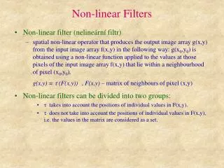
Non-linear Filters • Non-linear filter (nelineární filtr) • spatial non-linear operator that produces the output image array g(x,y) from the input image array f(x,y) in the following way: g(x0,y0) is obtained using a non-linear function applied to the values at those pixels of the input image array f(x,y) that lie within a neighbourhood of pixel (x0,y0). g(x,y) = t (F(x,y)) , F(x,y) – matrix of neighbours of pixel (x,y) • Non-linear filters can be divided into two groups: • t takes into account the positions of individual values in F(x,y). • t does not take into account the positions of individual values in F(x,y), i.e. the values in the matrix are considered as a set.
Examples of Non-linear Filters • Minimum (maximum) filter g(x,y) = minimum (maximum) of all F(x,y) matrix values • positions in matrix F(x,y) are not taken into account • Median filter g(x,y) = median of all F(x,y) matrix values • the most useful non-linear filter • removes camera defects (hot pixels) • preserves edges but removes thin lines and sharp corners • positions in matrix F(x,y) are not taken into account • MaxMin 5x5 filter g(x,y) = if the difference between maximum and minimum of the outer 16 pixels is larger than a pre-defined threshold, then the given pixel is replaced by the maximum or minimum of the outer 16 pixels (the value to which it is closer is chosen), otherwise it is replaced by the average of the neighbouring 8 pixels
Non-linear Filter Properties • Non-linear filter drawbacks • More difficult to implement (more time consuming) than linear ones • Not easy to find corresponding transform in frequency domain • Change of the sequence of non-linear filters changes the result(e.g. Max3x3(Min3x3(f)) Min3x3(Max3x3(f)) ) • The same applies also to the sequence of linear and non-linear filters(e.g. Median3x3(Gauss3x3(f)) Gauss3x3(Median3x3(f)) ) • Non-linear filter advantages • Sometimes non-linear filters produce better results than linear ones(e.g. median filtering removes noise better than any smoothing)
Deconvolution • Deconvolution (dekonvoluce) • an iterative process of estimating an original image from a convolved image. Convolution: g(x,y) = f(x,y) h(x,y) Usually: g(x,y) – recorded image f(x,y) – original image h(x,y) – convolution kernel (e.g. PSF) • Non-blind deconvolution • Input: g(x,y), h(x,y) • Output: f(x,y) • Blind deconvolution • Input: g(x,y) • Output: f(x,y), ( h(x,y) )
Deconvolution: Simplest Methods • Non-blind deconvolution • Simplest method: Direct computation • f(x,y) = IFFT ( FFT (g(x,y)) / FFT (h(x,y)) ) • unfortunately produces bad results because of noise in thoseparts of OTF where signal level is low • Blind deconvolution • Simplest method in 3D: Nearest neighbour • f(x,y,z) = g(x,y,z) – c ( g(x,y,z-1) + g(x,y,z+1) ) • based on the fact that PSF is elongated along z-axis in opticalmicroscopy • not very good results • reduces SNR • invented for slow computers
Deconvolution: MLE Approach • Maximum-likelihood estimation (MLE) approach • the most used approach to deconvolution, it performs iterative estimation of the most probable original function l(x,y,z). • Non-blind MLE approach • Blind MLE approach • h(k+1)(x,y,z) is modified in each iteration (after each new guess) so that it satisfies specific constraints which are known a priori (derived from optical laws)
Deconvolution Examples • A small hollow bead imaged at 25 photons/voxel. • Top row: XY plane through the centre of the bead. • Bottom row: XZ planes. • Left pair: raw image. • Right pair: MLE restoration.