Download
1 / 5
60 likes | 290 Vues
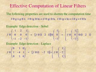
Effective Computation of Linear Filters. The following properties are used to shorten the computation time f g = g f, f (g h) = (f g) h, f (g + h) = f g + f h Example: Edge detection - Sobel Example: Edge detection - Laplace. Effective Computation of Linear Filters.

E N D
Effective Computation of Linear Filters The following properties are used to shorten the computation time f g = g f, f (g h) = (f g) h, f (g + h) = f g + f h Example: Edge detection - Sobel Example: Edge detection - Laplace
Effective Computation of Linear Filters Example: Sharpening filter Example: Smoothing - Gaussian
Effective Computation of Linear Filters Example: Smoothing combined with edge detection (LoG)
Linear Filters in Frequency Domain • Each linear filter in spatial domain (performed as convolution) has a corresponding filter in frequency domain (performed as multiplication) and vice versa. • Example: Low-pass filters • Ideal low-pass filter 1D: rectangle in frequency, k · sinc ax (sin ax / ax) in spatial domain 2D: rectangular box in frequency, k · sinc ax · sinc by in spatial domain 2D: cylinder in frequency, k · J1(sqrt(x2+y2)) in spatial domain • Non-weighted averaging 1D: rectangle in spatial, k · sinc awx in frequency domain 2D: rectangular box in spatial, k · sinc awx · sinc bwy in frequency domain 2D: cylinder in spatial, k · J1(sqrt(wx2+wy2)) in frequency domain • Weighted Gaussian averaging 1D: a · exp (-b · x2) in spatial, c · exp (-d · wx2) in frequency domain 2D: a · exp (-b · (x2+y2)) in spatial, c · exp (-d · (wx2+wy2)) in frequency
Linear Filters in Frequency Domain • Example: High-pass filters • Sobel 1D: 1st derivative in spatial, multiplication by -(iwx) in frequency domain 2D: 1st derivative in spatial, multiplication by -(iwd) in frequency domain • Laplace 1D: 2nd derivative in spatial, multiplication by -(wx2) in frequency 2D: 2nd derivative in spatial, multiplication by -(wx2+wy2) in frequency