Linear Filters
Linear Filters. Let . denote a bivariate time series with zero mean. . Suppose that the time series { y t : t T } is constructed as follows:. The time series { y t : t T } is said to be constructed from { x t : t T } by means of a Linear Filter .

Linear Filters
E N D
Presentation Transcript
Let denote a bivariate time series with zero mean.
Suppose that the time series {yt : tT} is constructed as follows: The time series {yt : t T} is said to be constructed from {xt : tT} by means of a Linear Filter.
Thus the spectral density of the time series {yt : tT} is:
Comment A: is called the Transfer function of the linear filter. is called the Gain of the filter while is called the Phase Shift of the filter.
Definition: = Squared Coherency function Note:
Comment B: = Squared Coherency function. if {yt : t T} is constructed from {xt : t T} by means of a linear filter
Let denote a bivariate time series with zero mean. Suppose that the time series {yt : tT} is constructed as follows: t = ..., -2, -1, 0, 1, 2, ... The noise {vt : tT} is independent of the series {xt : tT} (may be white)
The autocovariance function of the filtered series with added noise
continuing Thus the spectral density of the time series {yt : tT} is:
Thus = Squared Coherency function. Noise to Signal Ratio
Consider the Linear Filter of the time series {Xt : tT}: where and = the Transfer function of the filter.
{at : tT} is called the impulse response function of the filter since if X0 =1and Xt = 0 for t ≠ 0, then : for tT Xt at Linear Filter
Hence {DYt} and {DXt} are related by the same Linear Filter. Definition The Linear Filter is said to be stable if : converges for all |B| ≤1.
Many physical systems whose output is represented by Y(t) are modeled by the following differential equation: Where X(t) is the forcing function.
If X and Y are measured at discrete times this equation can be replaced by: where D = I-B denotes the differencing operator.
This equation can in turn be represented with the operator B. or where
This equation can also be written in the form as a Linear filter as Stability: It can easily be shown that this filter is stable if the roots of d(x) = 0 lie outside the unit circle.
Determining the Impulse Response function from the Parameters of the Filter:
Now or Hence
Equating coefficients results in the following conclusions: aj = 0 for j < b. aj - d1aj-1 - d2aj-2-...- draj-r= wj or aj= d1aj-1 + d2aj-2+...+ draj-r+ wj for b ≤ j ≤ b+s. and aj- d1aj-1 - d2aj-2-...- draj-r= 0 or aj = d1aj-1 + d2aj-2+...+ draj-r for j > b+s.
Thus the coefficients of the transfer function, a0, a1, a2,... , satisfy the following properties 1) b zeroesa0, a1, a2,..., ab-1 2) No pattern for the next s-r+1 values ab, ab+1, ab+2,..., ab+s-r 3) The remaining values ab+s-r+1, ab+s-r+2, ab+s-r+3,... follow the pattern of an rth order difference equation aj = d1aj-1 + d2aj-2+...+ dr aj-r
Example r =1, s=2, b=3, d1 = d a0 = a1 = a2 = 0 a3 = da2 + w0 = w0 a4 = da3 + w1 = dw0 + w1 a5 = da4 + w2 = d[dw0 + w1] + w2 = d2w0 + dw1 + w2 aj= daj-1 for j ≥ 6.
Recall the solution to the second order difference equation aj = d1aj-1 + d2aj-2 follows the following patterns: • Mixture of exponentials if the roots of • 1 - d1x - d2x2 = 0 are real. • 2) Damped Cosine wave if the roots to • 1 - d1x - d2x2 = 0 are complex. These are the patterns of the Impulse Response function one looks for when identifying b,r and s.
Estimation of the Impulse Response function, aj (without pre-whitening).
Suppose that {Yt : tT} and {Xt : t T}are weakly stationary time series satisfying the following equation: Also assume that {Nt : t T} is a weakly stationary "noise" time series, uncorrelated with {Xt : tT}. Then
Suppose that for s > M, as= 0. Then a0, a1, ... ,aM can be found solving the following equations:
If the Cross autocovariance function, sXY(h), and the Autocovariance function, sXX(h), are unknown they can be replaced by their sample estimates CXY(h) and CXX(h), yeilding estimates of the impluse response function
In matrix notation this set of linear equations can be written:
If the Cross autocovariance function, sXY(h), and the Autocovariance function, sXX(h), are unknown they can be replaced by their sample estimates CXY(h) and CXX(h), yeilding estimates of the impluse response function
Estimation of the Impulse Response function, aj (with pre-whitening).
Suppose that {Yt : tT} and {Xt : t T}are weakly stationary time series satisfying the following equation: Also assume that {Nt : t T} is a weakly stationary "noise" time series, uncorrelated with {Xt : tT}.
In addition assume that {Xt : t T}, the weakly stationary time series has been identified as an ARMA(p,q) series, estimated and found to satisfy the following equation: b(B)Xt=a(B)ut where {ut: t T} is a white noise time series. Then [a(B)]-1b(B)Xt= ut transforms the Time series {Xt : tT} into the white noise time series{ut : t T}.
This process is called Pre-whitening the Input series. Applying this transformation to the Output series {Yt : tT} yeilds:
or where and
In this case the equations for the impulse response function - a0, a1, ... ,aM - become (assuming that for s > M, as= 0):
Summary Identification and Estimation of Box-Jenkins transfer model

