Learn Discrete Probability Distribution with CK-12 FlexBook

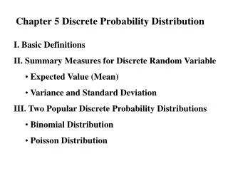
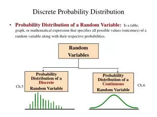
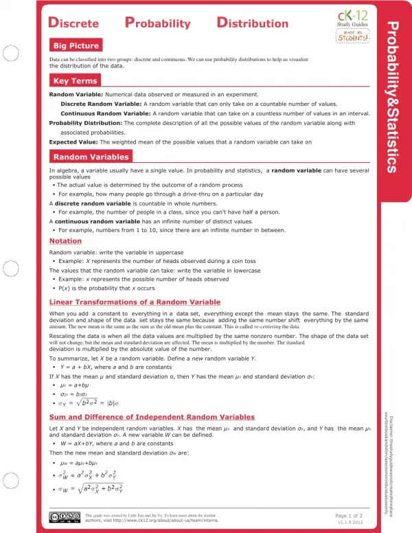
1. Discrete Probability Distribution Probability&Statistics Study Guides Big Picture Data can be classified into two groups: discrete and continuous. We can use probability distributions to help us visualize the distribution of the data. Key Terms Random Variable: Numerical data observed or measured in an experiment. Discrete Random Variable: A random variable that can only take on a countable number of values. Continuous Random Variable: A random variable that can take on a countless number of values in an interval. Probability Distribution: The complete description of all the possible values of the random variable along with associated probabilities. Expected Value: The weighted mean of the possible values that a random variable can take on Random Variables In algebra, a variable usually have a single value. In probability and statistics, a random variable can have several possible values • The actual value is determined by the outcome of a random process • For example, how many people go through a drive-thru on a particular day A discrete random variable is countable in whole numbers. • For example, the number of people in a class, since you can’t have half a person. A continuous random variable has an infinite number of distinct values. • For example, numbers from 1 to 10, since there are an infinite number in between. Notation Random variable: write the variable in uppercase • Example: X represents the number of heads observed during a coin toss The values that the random variable can take: write the variable in lowercase • Example: x represents the possible number of heads observed • P(x) is the probability that x occurs Linear Transformations of a Random Variable When you add a constant to everything in a data set, everything except the mean stays the same. The standard deviation and shape of the data set stays the same because adding the same number shift everything by the same amount. The new mean is the same as the sum as the old mean plus the constant. This is called re-centering the data. Rescaling the data is when all the data values are multiplied by the same nonzero number. The shape of the data set will not change, but the mean and standard deviation are affected. The mean is multiplied by the number. The standard deviation is multiplied by the absolute value of the number. To summarize, let X be a random variable. Define a new random variable Y. •  Y = a + bX, where a and b are constants If X has the mean μ and standard deviation σ, then Y has the mean μY and standard deviation σY: •  μY = a+bμ •  σ2Y = b2σ2 •  yourtextbookandisforclassroomorindividualuseonly. Sum and Difference of Independent Random Variables Disclaimer:thisstudyguidewasnotcreatedtoreplace Let X and Y be independent random variables. X has the mean μX and standard deviation σX, and Y has the mean μY and standard deviation σY. A new variable W can be defined. •  W = aX+bY, where a and b are constants Then the new mean and standard deviation σW are: •  μW = aμX+bμY •  •  Page 1 of 2 This guide was created by Lizhi Fan and Jin Yu. To learn more about the student authors, visit http://www.ck12.org/about/about-us/team/interns. v1.1.9.2012

2. Discrete Probability Distribution cont. Probability Distribution Probability Distribution for Probability distributions can be shown in a graph or table • Shows all the values a random variable can have and the Observing Heads in a 2-Coin Toss probability that each value will happen • Must satisfy two conditions: x P(x) 1. P(x) ≥ 0 for all values of X 0 ¼ 1 ½ 2. ΣP(x) = 1 for all values of X 2 ¼ Probability Example Let X be the number of heads observed when tossing two coins. Sample space: {HH, HT, TH, TT} So x = 0, 1, 2 • Means 0, 1, or 2 heads can be observed Characteristics • Mean (μ): an average value representing a central point of the distribution • Standard deviation (σ): how spread out the values are • Median: middle value • Mode: most common value Expected Value The expected value is the expected average outcome of an experiment. To find the expected value of X: 1. Find the probability P(x) of each possible outcome happening 2. Multiply the probability of each outcome by its value x 3. Add them all together: μ = E(x) = ΣxP(x) Standard Deviation The standard deviation is found by: • The sum Σ is taken over the entire sample space. The variance is the square of the standard deviation: Notes Page 2 of 2