Unit Hydrographs
Unit Hydrographs. Transforming the Runoff. Unit Hydrograph Theory. Moving water off of the watershed… A mathematical concept Linear in nature Uses convolution to transform the excess precipitation to streamflow…. Necessary for a single basin. Unit Hydrographs. Excess Precip. Model.

Unit Hydrographs
E N D
Presentation Transcript
Unit Hydrographs Transforming the Runoff
Unit Hydrograph Theory • Moving water off of the watershed… • A mathematical concept • Linear in nature • Uses convolution to transform the excess precipitation to streamflow….
Necessary for a single basin Unit Hydrographs Excess Precip. Model Excess Precip. Basin “Routing” UHG Methods Runoff Hydrograph Excess Precip. Stream and/or Reservoir “Routing” Downstream Hydrograph Runoff Hydrograph The Basic Process
Unit Hydrograph Theory • Sherman - 1932 • Horton - 1933 • Wisler & Brater - 1949 - “the hydrograph of surface runoff resulting from a relatively short, intense rain, called a unit storm.” • The runoff hydrograph may be “made up” of runoff that is generated as flow through the soil (Black, 1990).
Unit Hydrograph “Lingo” • Duration • Lag Time • Time of Concentration • Rising Limb • Recession Limb (falling limb) • Peak Flow • Time to Peak (rise time) • Recession Curve • Separation • Base flow
Graphical Representation Duration of excess precip. Lagtime Timeofconcentration Baseflow
Methods of Developing UHG’s • From Streamflow Data • Synthetically • Snyder • SCS • Time-Area (Clark, 1945) • “Fitted” Distributions
Unit Hydrograph • The hydrograph that results from 1-inch of excess precipitation (or runoff) spread uniformly in space and time over a watershed for a given duration. • The key points : • 1-inch of EXCESS precipitation • Spread uniformly over space - evenly over the watershed • Uniformly in time - the excess rate is constant over the time interval • There is a given duration
Derived Unit Hydrograph • Rules of Thumb : • … the storm should be fairly uniform in nature and the excess precipitation should be equally as uniform throughout the basin. This may require the initial conditions throughout the basin to be spatially similar. • … Second, the storm should be relatively constant in time, meaning that there should be no breaks or periods of no precipitation. • … Finally, the storm should produce at least an inch of excess precipitation (the area under the hydrograph after correcting for baseflow).
Separation of Baseflow • ... generally accepted that the inflection point on the recession limb of a hydrograph is the result of a change in the controlling physical processes of the excess precipitation flowing to the basin outlet. • In this example, baseflow is considered to be a straight line connecting that point at which the hydrograph begins to rise rapidly and the inflection point on the recession side of the hydrograph. • the inflection point may be found by plotting the hydrograph in semi-log fashion with flow being plotted on the log scale and noting the time at which the recession side fits a straight line.
Sample Calculations • In the present example (hourly time step), the flows are summed and then multiplied by 3600 seconds to determine the volume of runoff in cubic feet. If desired, this value may then be converted to acre-feet by dividing by 43,560 square feet per acre. • The depth of direct runoff in feet is found by dividing the total volume of excess precipitation (now in acre-feet) by the watershed area (450 mi2 converted to 288,000 acres). • In this example, the volume of excess precipitation or direct runoff for storm #1 was determined to be 39,692 acre-feet. • The depth of direct runoff is found to be 0.1378 feet after dividing by the watershed area of 288,000 acres. • Finally, the depth of direct runoff in inches is 0.1378 x 12 = 1.65 inches.
Again - Summing Flows Continuous process represented with discrete time steps
Obtain UHG Ordinates • The ordinates of the unit hydrograph are obtained by dividing each flow in the direct runoff hydrograph by the depth of excess precipitation. • In this example, the units of the unit hydrograph would be cfs/inch (of excess precipitation).
Determine Duration of UHG • The duration of the derived unit hydrograph is found by examining the precipitation for the event and determining that precipitation which is in excess. • This is generally accomplished by plotting the precipitation in hyetograph form and drawing a horizontal line such that the precipitation above this line is equal to the depth of excess precipitation as previously determined. • This horizontal line is generally referred to as the F-index and is based on the assumption of a constant or uniform infiltration rate. • The uniform infiltration necessary to cause 1.65 inches of excess precipitation was determined to be approximately 0.2 inches per hour.
Estimating Excess Precip. 0.8 0.7 0.6 0.5 Uniform loss rate of 0.2 inches per hour. Precipitation (inches) 0.4 0.3 0.2 0.1 0 0 1 2 3 4 5 6 7 8 9 10 11 12 13 14 15 16 17 18 19 Time (hrs.)
Changing the Duration • Very often, it will be necessary to change the duration of the unit hydrograph. • If unit hydrographs are to be averaged, then they must be of the same duration. • Also, convolution of the unit hydrograph with a precipitation event requires that the duration of the unit hydrograph be equal to the time step of the incremental precipitation. • The most common method of altering the duration of a unit hydrograph is by the S-curve method. • The S-curve method involves continually lagging a unit hydrograph by its duration and adding the ordinates. • For the present example, the 6-hour unit hydrograph is continually lagged by 6 hours and the ordinates are added.
Develop S-Curve Continuous 6-hour bursts
Convert to 1-Hour Duration • To arrive at a 1-hour unit hydrograph, the S-curve is lagged by 1 hour and the difference between the two lagged S-curves is found to be a 1 hour unit hydrograph. • However, because the S-curve was formulated from unit hydrographs having a 6 hour duration of uniformly distributed precipitation, the hydrograph resulting from the subtracting the two S-curves will be the result of 1/6 of an inch of precipitation. • Thus the ordinates of the newly created 1-hour unit hydrograph must be multiplied by 6 in order to be a true unit hydrograph. • The 1-hour unit hydrograph should have a higher peak which occurs earlier than the 6-hour unit hydrograph.
Average Several UHG’s • It is recommend that several unit hydrographs be derived and averaged. • The unit hydrographs must be of the same duration in order to be properly averaged. • It is often not sufficient to simply average the ordinates of the unit hydrographs in order to obtain the final unit hydrograph. A numerical average of several unit hydrographs which are different “shapes” may result in an “unrepresentative” unit hydrograph. • It is often recommended to plot the unit hydrographs that are to be averaged. Then an average or representative unit hydrograph should be sketched or fitted to the plotted unit hydrographs. • Finally, the average unit hydrograph must have a volume of 1 inch of runoff for the basin.
Synthetic UHG’s • Snyder • SCS • Time-area
Snyder • Since peak flow and time of peak flow are two of the most important parameters characterizing a unit hydrograph, the Snyder method employs factors defining these parameters, which are then used in the synthesis of the unit graph (Snyder, 1938). • The parameters are Cp, the peak flow factor, and Ct, the lag factor. • The basic assumption in this method is that basins which have similar physiographic characteristics are located in the same area will have similar values of Ct and Cp. • Therefore, for ungaged basins, it is preferred that the basin be near or similar to gaged basins for which these coefficients can be determined.
The final shape of the Snyder unit hydrograph is controlled by the equations for width at 50% and 75% of the peak of the UHG: Final Shape
Triangular Representation The 645.33 is the conversion used for delivering 1-inch of runoff (the area under the unit hydrograph) from 1-square mile in 1-hour (3600 seconds).
484 ? Comes from the initial assumption that 3/8 of the volume under the UHG is under the rising limb and the remaining 5/8 is under the recession limb.
Duration & Timing? Again from the triangle L = Lag time For estimation purposes :
Time of Concentration • Regression Eqs. • Segmental Approach
A Regression Equation where : Tlag = lag time in hours L = Length of the longest drainage path in feet S = (1000/CN) - 10 (CN=curve number) %Slope = The average watershed slope in %
Segmental Approach • More “hydraulic” in nature • The parameter being estimated is essentially the time of concentration or longest travel time within the basin. • In general, the longest travel time corresponds to the longest drainage path • The flow path is broken into segments with the flow in each segment being represented by some type of flow regime. • The most common flow representations are overland, sheet, rill and gully, and channel flow.
A Basic Approach Sorell & Hamilton, 1991 McCuen (1989) and SCS (1972) provide values of k for several flow situations (slope in %)
Triangular Shape • In general, it can be said that the triangular version will not cause or introduce noticeable differences in the simulation of a storm event, particularly when one is concerned with the peak flow. • For long term simulations, the triangular unit hydrograph does have a potential impact, due to the shape of the recession limb. • The U.S. Army Corps of Engineers (HEC 1990) fits a Clark unit hydrograph to match the peak flows estimated by the Snyder unit hydrograph procedure. • It is also possible to fit a synthetic or mathematical function to the peak flow and timing parameters of the desired unit hydrograph. • Aron and White (1982) fitted a gamma probability distribution using peak flow and time to peak data.
Hypothetical Example • A 190 mi2 watershed is divided into 8 isochrones of travel time. • The linear reservoir routing coefficient, R, estimated as 5.5 hours. • A time interval of 2.0 hours will be used for the computations.
Rule of Thumb R - The linear reservoir routing coefficient can be estimated as approximately 0.75 times the time of concentration.