Root Locus Analysis (3)
Root Locus Analysis (3). Hany Ferdinando Dept. of Electrical Eng. Petra Christian University. General Overview. This section explain how to use the Root Locus method to design compensator The compensator is lead and lag compensator Students need some basic geometry for precision drawing


Root Locus Analysis (3)
E N D
Presentation Transcript
Root Locus Analysis (3) Hany Ferdinando Dept. of Electrical Eng. Petra Christian University
General Overview • This section explain how to use the Root Locus method to design compensator • The compensator is lead and lag compensator • Students need some basic geometry for precision drawing • Pre-requisite: student has to understand how to plot Root Locus in complex plane
What is compensator • Compensation is the modification of the system dynamic to satisfy the given specification • Three compensators: lead, lag and lag-lead compensator • The lag-lead compensator will not be discussed • The compensator adds zero and pole to the system
Effects of the additional pole • It pulls the root locus to the right • It tends to lower the system’s relative stability • It slows down the settling time
Effects of the additional zeros • It pulls the root locus to the left • It tends to make the system more stable • It speeds up the settling time
Proof Proof that If R1C1 > R2C2 then it is lag network, otherwise it is lead network
Lead Compensator (1) Consider s = -1 ± j√3 Based on the closed-loop poles, z = 0.5, wn = 2 rad/s and Static velocity error (Kv) = 2s-1 Proof it!!
Lead Compensator (2) Problem: It is desired to modify the closed-loop poles so that the wn = 4 rad/s without changing the damping ratio z
Lead Compensator (3) For the wn = 4 rad/s without changing the damping ratio z, the desired closed-loop poles are inline with the line between the origin and the closed-loop poles of the system s = -2 ± j2√3
Lead Compensator (4) If G(s) is the open-loop transfer function, then the open-loop of compensated system is How to find a and T????
Lead Compensator (5) Desired closed-loop pole A P /2 /2 C B D O PB is the bisector between PA and PO f is the desired angle
Lead Compensator (6) Angle of at s = -2+j√3 is -210o Therefore the f is 30o From the previous slide method, the point C and D is approximately -5.4 and -2.9 You can try it by yourself!!
Lead Compensator (7) From the previous slide, you can calculate the T, aT and all Rs and Cs until you get: where K = 4Kc K = 18.7916
Lead Compensator (8) Compensated open-loop transfer function is with Gc(s) is Find the value for all Rs and Cs in the circuit
Lag Compensator (1) Consider s = -0.3307 ± j0.5864 Based on the closed-loop poles, z = 0.491, wn = 0.673 rad/s and Static velocity error (Kv) = 0.53s-1 Proof it!!
Lag Compensator (2) Problem: It is desired to increase the Kv to about 5s-1 without appreciably changing the location of the dominant closed-loop poles
Lag Compensator (3) The new Kv is about 10 times of the old Kv, therefore the b (a in the Lead Compensator) is set to 10. The zero of the compensator is also 10 times of the pole. We get K = 1.06Kc
Lag Compensator (4) The Root Locus plot of the compensated system is very close to the uncompensated one. Therefore, we need Matlab to help us. The new dominant closed-loop pole with the same z is -0.31±j0.55 (from Matlab). The gain K is 1.0235
Find the pole in complex plane To find the desired dominant complex pole in the Root Locus plot, one can use rlocfind(num,den) function. Output of this function is the selected pole and the gain at that pole. When this function is called, there is a pointer one can use to select a pole in the complex plane. Usually, the Root Locus is drawn first.
Next… Bode diagram as a tool for frequency response analysis is the next topic. Prepare yourself for this…