Root Locus Design
Root Locus Design. 5. ▶ Relationship between Root Locus and Time Domain. ▶ Compensation. ▶ Uncompensated System. ▶ Cascade PI Compensated System. ▶ Cascade Lag Compensation. ▶ Cascade Lead Compensation. ▶ Cascade Lag-Lead Compensation. ▶ Rate Feedback Compensation (PD).

Root Locus Design
E N D
Presentation Transcript
▶ Relationship between Root Locus and Time Domain ▶ Compensation ▶ Uncompensated System ▶ Cascade PI Compensated System ▶ Cascade Lag Compensation ▶ Cascade Lead Compensation ▶ Cascade Lag-Lead Compensation ▶ Rate Feedback Compensation (PD) ▶ Proportional-Integral-Derivative Compensation
◎ Relationship between Root Locus and Time Domain ― Second-order control system
If the damping ratio is between zero and one, complex conjugate poles of result. Figure. Complex conjugate poles
※ When the closed-loop poles are moved, the rise time and settling time of the dominant roots change Figure. Changes in damping ratio and undamped natural frequency Figure. Rise time versus damping ratio Figure. Settling time versus damping ratio
Figure. Figure. Therefore, if the damping ratio is fixed and we want to reduce rise time and settling time, then the root locus design must cause , and therefore the relative stability to be as large as possible. Ex) the unit step response of a second-order underdamped system
Figure. Figure. The design strategy : maximize the relative stability of the dominant poles when that is possible and to make the damping ratio 0.707 for the dominant poles when that choice is possible.
◎ Compensation Configurations a) Series (cascade) compensation : The most commonly used system configuration with the controller placed in series with the controlled process. b) Feedback compensation : The controller is placed in the minor feedback path.
c) State feedback compensation : A system that generates the control signal by feeding back the state variables through constant real gains. The problem with state-feedback control is that for high-order systems, the large number of state variables involved would require a large number of tranducers to sense the state variables for feedback. Thus actual implementation of the state-feedback control scheme may be costly or impractical. Even for low- order systems, often not all the state variables are directly accessible, and an observer or estimator may be necessary to create the estimated state variables from measurem- ents of the output variables. d) Series-feedback compensation : The series-feedback compensation for which a series controller and a feedback controller are used.
▶ The feedforward controller is placed in series with the closed-loop system, which has a controller in the forward path. ▶ The feedforward controller is placed in parallel with the forward path. : The key to the feedforward compensation is that the controller is not in the loop of the system, so that it does not affect the roots of the characteristic equation of the original system. The poles and zeros of may be selected to add or cancel the poles and zeros of the closed -loop system transfer function. e) Feedforward compensation
◎ Uncompensated System Special Ex) Figure. Root locus
For each the ramp error coefficient is As increases, the ramp error coefficient increases, the ramp error decreases, and the dominant roots become more lightly damped.
Figure. Ramp error Figure. Step response
※ Second-Order Plant Models The uncompensated system is type 1. The uncompensated system is type 0. ※ Each compensator can now be applied to the type 1 or type 0 model to approximate how each compensator affects the dominant roots of the actual system
※ The PI compensator thus adds a pole at and a zero at to the open-loop transmittance . ◎ Cascade PI Compensation The cascade PI compensator has a transmittance of the form → System type increases by 1 Hence, for a stable design, steady state error performance is improved.
For the compensated system with open-loop transmittance As the compensator contributes a pole at and a zero at ( is the centroid for the uncompensated system) The compensated system has the same root locus asymptotic angles as does the uncompensated one. However, the centroid of the asymptotes does change. ※ For a positive , is moved to the right, tending to reduce relative stability from that of the uncompensated feedback system by an amount proportional to .
If we let while varies, The equivalent required to obtain the root locus for variable is Ex) Figure. PI compensator (type 1 system)
For there are closed-loop poles at ※ The maximum relative stability is a value so that all three poles have the same real part (― c). Figure. Root locus for variable If the roots are and In order to determine the best value of with , equate the characteristic polynomial
By equating the coefficients By equating the coefficients Finally, can be obtained by equating the coefficients Figure. Compares values of for various values of
Ex) Figure. PI compensator (type 0 system) If , a root locus for variable
Special Ex) If , then the compensator for variable
The value of for maximum relative stability is . Figure. Root locus The closed-loop poles are at . The relative stability is
→ Not increase the system type number. However, steady state error performance can be improved ◎ Cascade Lag Compensation The cascade lag compensator has a transmittance of the form ※ where , and are positive constants and → The compensator zero is to the left of the compensator pole.
The error coefficient for an uncompensated system is For a lag compensated system The ratio of the error coefficient The centroid for a cascade lag compensated system moves to the right by
The error coefficient increases by the factor If approaches infinity, the cascade lag compensator becomes cascade PI As with the PI compensator, maximum relative stability is a reasonable goal, and we should select for a type 1 plant and for a type 0 plant.
If the second-order model is used with then . Suppose we want to increase the error coefficient by a factor of 10 compared to the uncompensated case. Then we should choose and . Ex) Consider the type 1.
The value of for maximum relative stability can be found by trial and error using a root-solving routine. With Pole → Figure. Root locus for variable There is a zero at due to the lag compensator zero. Figure. Root locus for variable
The ramp error coefficient is now , so the steady state ramp error is . Figure. Ramp error Figure. Step response The ramp error and step response for the lag compensated system are quite close to those for the PI compensated system. The compensator is therefore
Select for the uncompensated system. • Calculate and for the dominant poles. 4. Examine the root locus for variable and adjust for acceptable stability. It may be best to choose for maximum relative stability. 5. Vary , and as required to meet design requirements. ※ To summarize, the design procedure for lag compensation is 2. For a type 1 system, begin with For a type 0 system, begin with 3. In order to increase the error coefficient by a factor of , select
※ where , and are positive constants and → The compensator pole is to the left of the zero. ◎ Cascade Lead Compensation The cascade lead compensator has a transmittance of the form The centroid moves to the left by ( the asymptote angles are unchanged ) → The root locus moves to the left.
with , where . The performance of the cascade lead compensator is more easily evaluated by replacing For a lead compensated system The ratio of the error coefficient
Ex) To simplify the transfer function,
The root locus for adjustable requires plotting, Figure. Root locus for variable
Select for the uncompensated system. 2. Select . A large value may create problems in realizing an circuit with widely separated poles and zeros, so the range of to is normal. 3. Select . This maintains steady state accuracy compared to the uncompensated case. 4. Select for maximum relative stability. 5. Vary , and as required to meet design requirements. ※ To summarize, the design procedure for lead compensation is
The root locus for adjustable requires plotting, The closed-loop transfer function is,
has been selected to be . If we choose , as we did for the lag compensator, then to maintain the same ramp error coefficient as for the uncompensated case , so
Figure. Root locus for variable If , the closed-loop poles are at The relative stability of is higher than for the uncompensated case ( ). Figure. Root locus for variable
Figure. Ramp error Figure. Step response Compared to the uncompensated system, the responses are better (less overshoot), while the steady state ramp error is unchanged. The goals of lead compensation are thus met. The compensator is therefore
◎ Cascade Lag-Lead Compensation A cascade lag compensator improves steady state. A cascade lead compensator improves relative stability. The best attributes of both compensators can be combined The design is simplified if the pole-zero ratios are set by The ratio of error coefficients becomes
Select for the uncompensated system. • Calculate and for the dominant poles. If the pole-zero ratios are as above, the compensator becomes ( for ) ※ In order to design the lag-lead compensator, For the lag part of the compensator 2. For a type 1 system, begin with For a type 0 system, begin with 3. In order to increase the error coefficient by a factor of , select
4. Apply only the lag compensator to the plant, examine the root locus for variable and adjust for acceptable stability. It may be best to choose for maximum For the lead part of the compensator • Select . This maintains steady state accuracy compared to the lag case. 6. Apply only te lead compensator to the plant, with and select for maximum relative stability. For the lag-lead compensator 7. Vary and as required to meet design requirements.
Ex) At this point in the design process, and the ramp error coefficient is . And closed-loop poles are And closed-loop zeros are
Figure. Ramp error (K=30) Figure. Step response (K=30) Figure. Ramp error (K=60) Figure. Step response (K=60)
Figure. Root locus Due to the closed-loop poles at , the cascade lag-lead compensated system with has a slower response than the cascade lag compensated system. (the settling time is 9.8 sec compared to 8.7 sec) The root locus for variable is easy to obtain by applying a computer to
With , the closed-loop poles are at The adjustment of step 7 results in
◎ Rate Feedback Compensation (PD) ※ Feedback compensated system Feedback rate compensation has ※ The zero added ( ) This compensator has an output that is proportional to its input and an output that is the derivative of its input. Proportional derivative (PD) compensator