Download

1 / 48
490 likes | 801 Vues
INC341 Design with Root Locus. Lecture 9. 2 objectives for desired response. Improving transient response Percent overshoot, damping ratio, settling time, peak time Improving steady-state error Steady state error. Gain adjustment.

E N D
INC341Design with Root Locus Lecture 9
2 objectives for desired response • Improving transient response • Percent overshoot, damping ratio, settling time, peak time • Improving steady-state error • Steady state error
Gain adjustment • Higher gain, smaller steady stead error, larger percent overshoot • Reducing gain, smaller percent overshoot, higher steady state error
Compensator • Allows us to meet transient and steady state error. • Composed of poles and zeros. • Increased an order of the system. • The system can be approx. to 2nd order using some techniques.
Point A and B have the same damping ratio. Starting from point A, cannot reach a faster response at point B by adjusting K. Compensator is preferred. Improving transient response
Compensator configulations Cascade Compensator Feedback Compensator The added compensator can change a pattern of root locus
Types of compensator • Active compensator • PI, PD, PID use ofactive components, i.e.,OP-AMP • Require power source • ss error converge to zero • Expensive • Passive compensator • Lag,Leaduse ofpassive components, i.e., R L C • No need of power source • ss error nearly reaches zero • Less expensive
Improving steady-state error Placing apole at theorigin to increase system order; decreasing ss error as a result!!
The pole at origin affects the transeint response adds a zero close to the pole to get an ideal integral compensator
Example Choose zero at -1 Damping ratio = 0.174 in both uncompensated and PI cases
Draw root locus without compensator • Draw a straight line of damping ratio • EvaluateK from the intersection point • From K, find the last pole (at -11.61) • Calculate steady-state error
Finding an intersection between damping ratio line and root locus • Damping ratio line has an equation: where a = real part, b = imaginary part of the intersection point, • Summation of angle from open-loop poles and zeros to the point is 180 degrees
Use the formula to get the real and imaginary part of the intersection point and get • Magnitude of open loop system is 1 No open loop zero
Draw root locus with compensator (system order is up by 1--from 3rd to 4th) • Needs complex poles corresponding to damping ratio of 0.174 (K=158.2) • From K, find the 3rd and 4th poles (at -11.55 and -0.0902) • Pole at -0.0902 can do phase cacellation with zero at -1 (3th order approx.) • Compensated system and uncompensated system have similar transient response (closed loop poles and K are aprrox. The same)
Lag Compensator • Build from passive elements • Improve ss error by a factor of Zc/Pc • To improve both transient and ss responses, put pole and zero close to the origin
Uncompensated system With lag compensation (root locus remains the same)
Example With damping ratio of 0.174, add lag Compensator to improvesteady-state error by a factor of 10
Step I: find an intersection of root locus and damping ratio line (-0.694+j3.926 withK=164.56) Step II:findKp = lim G(s) as s0 (Kp=8.228) Step III:steady-state error =1/(1+Kp)= 0.108 Step IV:want to decrease error down to0.0108 [Kp = (1 – 0.0108)/0.0108 = 91.593] Step V: require a ratio of compensator zero to pole as91.593/8.228 = 11.132 Step VI: choose apole at0.01, the corresponding Zero will be at 11.132*0.01 = 0.111
3rd order approx. for lag compensator (= uncompensated system) making Same transient response but 10 times Improvement in ss response!!!
If we choose acompensator pole at 0.001 (10 times closer to the origin), we’ll get a compensatorzero at0.0111 (Kp=91.593) New compensator: 4th pole is at -0.01 (compared to -0.101) producing a longer transient response.
SS response improvement conclusions • Can be done either by PI controller (pole at origin) or lag compensator (pole closed to origin). • Improving ss error without affecting the transient response. • Next step is to improve the transient response itself.
Improving Transient Response • Objective is to • Decrease settling time • Get a response with a desired %OS (damping ratio) • Techniques can be used: • PD controller (ideal derivative compensation) • Lead compensator
Ideal Derivative Compensator • So called PD controller • Compensator adds a zero to the system at –Zc to keep a damping ratio constant with a faster response
(a) Uncompensated system, (b) compensator zero at -2 (d) compensator zero at -3, (d) compensator zero at -4 Indicate peak time Indicate settling time
Settling time & peak time: (b)<(c)<(d)<(a) • %OS: (b)=(c)=(d)=(a) • ss error: compensated systems has lower value than uncompensated one cause improvement in transient response always yields an improvement in ss error
Example design a PD controller to yield 16% overshoot with a threefold reduction in settling time
Step I: calculate a corresponding damping ration (16% overshoot = 0.504 damping ratio) • Step II: search along the damping ratio line for an odd multiple of 180 (at -1.205±j2.064) and corresponding K (43.35) • Step III: find the 3rd pole (at -7.59) which is far away from the dominant poles 2nd order approx. works!!!
More details in step II and III Characteristic equation:
Step IV: evaluate a desired settling time: • Step V: get corresponding real and imagine number of the dominant poles (-3.613 and -6.193)
Location of poles as desired is at -3.613±j6.192
Step VI: summation of angles at the desired pole location, -275.6, is not an odd multiple of 180 (not on the root locus) need to add a zero to make the sum of 180. • Step VII: the angular contribution for the point to be on root locus is +275.6-180=95.6 put a zero to create the desired angle
Compensator: (s+3.006) Might not have a pole-zero cancellation for compensated system
Lead Compensation Zeta2-zeta1=angular contribution
Example Design three lead compensators for the system that has30% OS and will reducesettling time down by a factor of 2.
Step I: %OS = 30% equaivalent todamping ratio = 0.358, Ѳ= 69.02 • Step II: Search along the line to find a point that gives 180 degree (-1.007±j2.627) • Step III: Find a corresponding K ( ) • Step IV: calculate settling time of uncompensated system • Step V: twofold reduction in settling time (Ts=3.972/2 = 1.986), correspoding real and imaginary parts are:
Step VI: let’s put a zero at -5 and find the net angle to the test point (-172.69) • Step VII: need a pole at the location giving 7.31 degree to the test point.
Note: check if the 2nd order approx. is valid for justify our estimates of percent overshoot and settling time • Search for 3rd and 4th closed-loop poles (-43.8, -5.134) • -43.8 is more than 20 times the real part of the dominant pole • -5.134 is close to the zero at -5 The approx. is then valid!!!