Root locus
Root locus. A technique enabling you to see how close-loop poles would vary if a parameter in the system is varied Can be used to design controllers or tuning controller parameters so as to move the dominant poles into the desired region.


Root locus
E N D
Presentation Transcript
Root locus • A technique enabling you to see how close-loop poles would vary if a parameter in the system is varied • Can be used to design controllers or tuning controller parameters so as to move the dominant poles into the desired region
Recall: step response specs are directly related to pole locations • Let p=-s+jwd • ts proportional to 1/s • Mp determined by exp(-ps/wd) • tr proportional to 1/|p| • It would be really nice if we can • Predict how the poles move when we tweak a system parameter • Systematically drive the poles to the desired region corresponding to desired step response specs
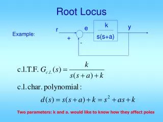
Root Locus k s(s+a) y e r Example: + - Two parameters: k and a. would like to know how they affect poles
The root locus technique • Obtain closed-loop TF and char eq d(s) = 0 • Rearrange terms in d(s) by collecting those proportional to parameter of interest, and those not; then divide eq by terms not proportional to para. to get this is called the root locus equation • Roots of n1(s) are called open-loop zeros, mark them with “o” in s-plane; roots of d1(s) are called open-loop poles, mark them with “x” in s-plane
The “o” and “x” marks falling on the real axis divide the real axis into several segments. If a segment has an odd total number of “o” and/or “x” marks to its right, then n1(s)/d1(s) evaluated on this segment will be negative real, and there is possible k to make the root locus equation hold. So this segment is part of the root locus. High light it. If a segment has an even total number of marks, then it’s not part of root locus. For the high lighted segments, mark out going arrows near a pole, and incoming arrow near a zero.
Let n=#poles=order of system, m=#zeros. One root locus branch comes out of each pole, so there are a total of n branches. M branches goes to the m finite zeros, leaving n-m branches going to infinity along some asymptotes. The asymptotes have angles (–p +2lp)/(n-m). The asymptotes intersect on the real axis at:
Imaginary axis crossing • Go back to original char eq d(s)=0 • Use Routh criteria special case 1 • Find k value to make a whole row = 0 • The roots of the auxiliary equation are on jw axis, give oscillation frequency, are the jw axis crossing points of the root locus • When two branches meet and split, you have breakaway points. They are double roots. d(s)=0 and d’(s) =0 also. Use this to solve for s and k. • Use matlab command to get additional details of root locus • Let num = n1(s)’s coeff vector • Let den = d1(s)’s coeef vector • rlocus(num,den) draws locus for the root locus equation • Should be able to do first 7 steps by hand.