Root Locus Technique and Eigenvalue Curves in Control Systems Analysis

DESCRIPTION

This document explores the root locus technique to analyze the behavior of eigenvalues in the s-plane as a parameter K varies. Using Example 5.1, we determine the roots of a polynomial and construct the root locus for specific values. It discusses key concepts such as breakaway points, asymptotes, and their influence on system stability. Additionally, using MATLAB functions like `rlocus` and `rlocfind`, we illustrate how to visualize the root locus and identify critical points of interest.

Download

1 / 3

May 08, 2026

Télécharger la présentation

Root Locus Technique and Eigenvalue Curves in Control Systems Analysis

An Image/Link below is provided (as is) to download presentation Download Policy: Content on the Website is provided to you AS IS for your information and personal use and may not be sold / licensed / shared on other websites without getting consent from its author. Content is provided to you AS IS for your information and personal use only. Download presentation by click this link. While downloading, if for some reason you are not able to download a presentation, the publisher may have deleted the file from their server. During download, if you can't get a presentation, the file might be deleted by the publisher.

E N D

Presentation Transcript

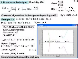
R ( s ) Kuo-95 (p.470) 5. Root-Locus Technique Curves of eigenvalues in the s-plane depending on K Example 5.1 n1=[1,3];a1=conv([1,5,0],[1,6]); a2=[1,2,2];p=roots(a2) d1=conv(a1,a2) rlocus(n1,d1) Roots: D1(s)=0 Zeros: N1(s)=0 5 parts ( D1(s) 5. order) Symmetricalwith respect to real axis
Intersect of the asymptotes: Routh tabulation (Example 3.1) k=35; a=polyadd(d1,k*n1);p=roots(a) Breakaway points: n1d=[1];d1d=[5,4*13,3*54,2*82,60]; a=polyadd(conv(n1d,d1),-conv(d1d,n1));roots(a)
ksi=0.6;wn=2;sg=-ksi*wn;w=wn*sqrt(1-ksi^2); hold on;plot([0,sg],[0,w]);hold off;rlocfind(n1,d1)