Root Locus Diagrams
Root Locus Diagrams. Professor Walter W. Olson Department of Mechanical, Industrial and Manufacturing Engineering University of Toledo. Outline of Today’s Lecture. Review The Block Diagram Components Block Algebra Loop Analysis Block Reductions Caveats Poles and Zeros


Root Locus Diagrams
E N D
Presentation Transcript
Root Locus Diagrams Professor Walter W. Olson Department of Mechanical, Industrial and Manufacturing Engineering University of Toledo
Outline of Today’s Lecture • Review • The Block Diagram • Components • Block Algebra • Loop Analysis • Block Reductions • Caveats • Poles and Zeros • Plotting Functions with Complex Numbers • Root Locus • Plotting the Transfer Function • Effects of Pole Placement • Root Locus Factor Responses
Block Diagrams Actuate Sense Disturbance • Throughout this course, we have used block diagrams to show different properties • Here, we will formalize the meaning of block diagrams Controller u Controller Plant Compute Plant/Process Input r Output y S S kr … State Controller y S S S S Sensor Prefilter D c1 c2 cn-1 cn x … z1 z2 zn zn-1 -K u S State Feedback -1 a1 a2 an-1 an … S S S
Components x The paths represent variable values which are passed within the system xG(s) x Blocks represent System components which are represented by transfer functions and multiply their input signal to produce an output G(s) x+y x Addition and subtraction of signals are represented by a summer block with the operation indicated on the arrow + + y x x Branch points occur when a value is placed on two lines: no modification is made to the signal x
Block Algebra Gx x G(x-z) Gx-z (G-H)x Gx Hx x x x x Gx G-H G G G G G G G H G Gx z Gx-z (G-H)x x x Gx Gx z x + + + + + - - - - - Gx G(x-z) z Gz z G
Loop Analysis(Very important slide!) Negative Feedback Y(s) R(s) E(s) Positive Feedback H(s) Y(s) R(s) E(s) H(s) B(s) G(s) B(s) + + + -
Loop Nomenclature Disturbance/Noise Reference Input R(s) Error signal E(s) Output y(s) Controller C(s) Plant G(s) Prefilter F(s) Open Loop Signal B(s) Sensor H(s) + + - - The plant is that which is to be controlled with transfer function G(s) The prefilter and the controller define the control laws of the system. The open loop signal is the signal that results from the actions of the prefilter, the controller, the plant and the sensor and has the transfer function F(s)C(s)G(s)H(s) The closed loop signal is the output of the system and has the transfer function
Caveats: Pole Zero Cancellations • Assume there were two systems that were connected as such • An astute student might note thatand then want to cancel the (s+1) term This would be problematic: if the (s+1) represents a true system dynamic, the dynamic would be lost as a result of the cancellation. It would also cause problems for controllability and observability. In actual practice, cancelling a pole with a zero usually leads to problems as small deviations in pole or zero location lead to unpredictable dynamics under the cancellation. Y(s) R(s)
Caveats: Algebraic Loops • The system of block diagrams is based on the presence of differential equation and difference equation • A system built such the output is directly connected to the input of a loop without intervening differential or time difference terms leads to improper block interpretations and an inability to simulate the model. • When this occurs, it is called an Algebraic Loop. Such loops are often meaningless and errors in logic. 2 + -
Gain, Poles and Zeros • The roots of the polynomial in the denominator, a(s), are called the “poles” of the system • The poles are associated with the modes of the system and these are the eigenvalues of the dynamics matrix in a state space representation • The roots of the polynomial in the numerator, b(s) are called the “zeros” of the system • The zeros counteract the effect of a pole at a location • The variable s is a complex number: • The value of G(0) is the zero frequency or steady state gain of the system
Plotting functions on the Complex Plane • Plotting functions on the complex plane is more complicated than the real plane because of unexpected forms that occur • Consider an equation such as • If z is limited to real numbers, z must be 1 for any n • BUT, this is not the case if z is allowed to be a complex number • if n = 3, then • If n = 4, then • Consider a function such as • If z were real, a hyperbola results • BUT, if z is a complex number, a totally different result occurs • Both a and b vary with results in surface rather than a curve • The result of the function could be either real or complex • Therefore, visualization is difficult
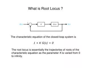
Root Locus • The root locus plot for a system is based on solving the system characteristic equation • The transfer function of a linear, time invariant, system can be factored as a fraction of two polynomials • When the system is placed in a negative feedback loop the transfer function of the closed loop system is of the form • The characteristic equation is • The root locus is a plot of this solution for positive real values of K • Because the solutions are the system modes, this is a powerful design tool • While we focus here on the gain, K, we can plot any parameter this way
Plotting a Transfer Function Root Locus • The path is determined from the open loop transfer function by varying the gain • ‘s’ as used in a transfer function is a complex number • Poles will be marked with X • Zeros with be marked with an O • Each path represents a branch of the transfer function in the complex plane • All paths • start at poles and • end at zeros • mirror across the real axis • There must be a zero for each pole • Those that are not shown on the plot are at infinity • Matlab command rlocus(sys)
Paths of the Transfer Function K=1 K=3 K=10 K=0.1
Paths of the Transfer Function • The real values of the gain move the poles along the root loci • Notice that the placement of the gain moved poles dictates the output response of the system • Poles in the right half plane are unstable responses K=1 K=3 K=10 K=0.1
The effect of placement on the root locus jw Imaginary axis jwd sin-1(z) wn Real Axis s s = -zwn • The magnitude of the vector to • pole location is the natural frequency • of the response, wn • The vertical component (the imaginary • part) is the damped frequency, wd • The angle away from the vertical is the • inverse sine of the damping ratio, z
Root Locus Factor Responses jw s A complete system will sum all of these effects that are present in the system’s response The dominating effects will be from the poles closest to the origin Real Axis
Example • A radar tracking antenna (Nise, 1995) has the position control transfer function of • The antenna must have a 5% settling time of less than 2 seconds with an over damped response.
Example • Current system can not meet either requirement with gain alone: • By adding a zero at -1.34, a pole at -11 and a gain of 271, we get • Is this the best controller?
Summary jw • Poles and Zeros • Plotting Functions with Complex Numbers • Root Locus • Plotting the Transfer Function • Effects of Pole Placement • Root Locus Factor Responses Imaginary axis jwd sin-1(z) wn Real Axis s s = -zwn Next: Bode Plots