Root-locus Design Method
Root-locus Design Method. Outline Build dynamic models Study the dynamic responses of a system Basic properties of feedback control How to design control systems Root-locus method Frequency-response method State-space method. Root-locus Design Method. Applications of the Guidelines

Root-locus Design Method
E N D
Presentation Transcript
Root-locus Design Method Outline • Build dynamic models • Study the dynamic responses of a system • Basic properties of feedback control • How to design control systems • Root-locus method • Frequency-response method • State-space method Northern Illinois University Summer 2005
Root-locus Design Method Applications of the Guidelines Consider the root locus of the characteristic equation 1+KG(s)=o, where Construct the root locus for various values of P. Northern Illinois University Summer 2005
Root-locus Design Method Applications of the Guidelines Case 2: P=4. Northern Illinois University Summer 2005
Root-locus Design Method Step 1: mark poles & zeros j 0 = pole = zero Northern Illinois University Summer 2005
Root-locus Design Method Step 2: draw locus on real axis to the left of an odd number of poles plus zeros: j 0 = pole = zero Northern Illinois University Summer 2005
Root-locus Design Method Step 3: Find the number of asymptotes and draw them number of asymptotes = n-m=3 - 1=2 Northern Illinois University Summer 2005
Root-locus Design Method Step 3: j 0 = pole = zero Northern Illinois University Summer 2005
Root-locus Design Method Step 4: Calculate departure and arrival angles j 0 = pole = zero Northern Illinois University Summer 2005
Root-locus Design Method Step 4: Calculate departure and arrival angles Draw a small circle around the double poles. Northern Illinois University Summer 2005
Root-locus Design Method Step 4: Calculate departure and arrival angles j 0 = pole = zero Northern Illinois University Summer 2005
Root-locus Design Method Step 5: Cross-over on the imaginary axis The characteristic equation is Build Routh array: For K>0, all roots are in LHP and do not cross imaginary axis. Northern Illinois University Summer 2005
Root-locus Design Method Step 6: estimate the locations of multiple roots, and find the arrival and departure angles at these locations. We found that G(s = -1.75+0.97j) and G(s = -1.75-0.97j) are not 180. Therefore, multiple roots are at s=0 only. Northern Illinois University Summer 2005
Root-locus Design Method Step 7: Sketch the locus j 0 = pole = zero Northern Illinois University Summer 2005
Root-locus Design Method Applications of the Guidelines Case 3: P=12 Northern Illinois University Summer 2005
Root-locus Design Method Step 1: mark poles & zeros j 0 = pole = zero Northern Illinois University Summer 2005
Root-locus Design Method Step 2: draw locus on real axis to the left of an odd number of poles plus zeros: j 0 = pole = zero Northern Illinois University Summer 2005
Root-locus Design Method Step 3: Find the number of asymptotes and draw them number of asymptotes = n-m=3 - 1=2 Northern Illinois University Summer 2005
Root-locus Design Method Step 3: j 0 = pole = zero Northern Illinois University Summer 2005
Root-locus Design Method Step 4: Calculate departure and arrival angles j 0 = pole = zero Northern Illinois University Summer 2005
Root-locus Design Method Step 4: Calculate departure and arrival angles Draw a small circle around the double poles. Northern Illinois University Summer 2005
Root-locus Design Method Step 4: Calculate departure and arrival angles j 0 = pole = zero Northern Illinois University Summer 2005
Root-locus Design Method Step 5: Cross-over on the imaginary axis The characteristic equation is Build Routh array: For K>0, all roots are in LHP and do not cross imaginary axis. Northern Illinois University Summer 2005
Root-locus Design Method Step 6: estimate the locations of multiple roots, and find the arrival and departure angles at these locations. All roots are on the locus. Multiple roots are at s=0, -2.31 and –5.18. Northern Illinois University Summer 2005
Root-locus Design Method Step 7: Sketch the locus j 0 = pole = zero Northern Illinois University Summer 2005
Root-locus Design Method Applications of the Guidelines Case 4: P=9 Northern Illinois University Summer 2005
Root-locus Design Method Step 1: mark poles & zeros j 0 = pole = zero Northern Illinois University Summer 2005
Root-locus Design Method Step 2: draw locus on real axis to the left of an odd number of poles plus zeros: j 0 = pole = zero Northern Illinois University Summer 2005
Root-locus Design Method Step 3: Find the number of asymptotes and draw them number of asymptotes = n-m=3 - 1=2 Northern Illinois University Summer 2005
Root-locus Design Method Step 3: j 0 = pole = zero Northern Illinois University Summer 2005
Root-locus Design Method Step 4: Calculate departure and arrival angles j 0 = pole = zero Northern Illinois University Summer 2005
Root-locus Design Method Step 4: Calculate departure and arrival angles Draw a small circle around the double poles. Northern Illinois University Summer 2005
Root-locus Design Method Step 4: Calculate departure and arrival angles j 0 = pole = zero Northern Illinois University Summer 2005
Root-locus Design Method Step 5: Cross-over on the imaginary axis The characteristic equation is Build Routh array: For K>0, all roots are in LHP and do not cross imaginary axis. Northern Illinois University Summer 2005
Root-locus Design Method Step 6: estimate the locations of multiple roots, and find the arrival and departure angles at these locations. All roots are on the locus. Repeated roots in the derivative indicates triple roots at s=-3. Northern Illinois University Summer 2005
Root-locus Design Method Step 6: 3 locus segments will approach at 120 wrt each other and depart with a 60 change relative to the arrival angles. Northern Illinois University Summer 2005
Root-locus Design Method Step 7: Sketch the locus j 0 = pole = zero Northern Illinois University Summer 2005
Root-locus Design Method Effects of the Third Pole (Summary) • Where size of P increases, the asymptote moves steadily to the left until it is out of sight. • When P is small and near the zero, the third pole has only modest distorting effect on the root locus. • When P increases, the third pole has increasingly distorting effect on the root locus. • When P is -9, triple multiple roots. • When P goes beyond -9, very distinct break-in and break-away points appear. • When P gets very large, the root locus approaches the circular locus of one zero and two poles. Northern Illinois University Summer 2005
Root-locus Design Method P=1 j 0 = pole = zero Northern Illinois University Summer 2005
Root-locus Design Method P=4 j 0 = pole = zero Northern Illinois University Summer 2005
Root-locus Design Method P=9 j 0 = pole = zero Northern Illinois University Summer 2005
Root-locus Design Method P=12 j 0 = pole = zero Northern Illinois University Summer 2005
Root-locus Design Method P>>12 j 0 = pole = zero Northern Illinois University Summer 2005
Root-locus Design Method Selecting Gain from the Root Locus The purpose of design is to select a particular gain K that meet the specifications for static and dynamic responses. Northern Illinois University Summer 2005
Root-locus Design Method Selecting Gain from the Root Locus To have a root at a particular location of the root locus for a certain K, both the phase and magnitude conditions have to be met. Phase condition: for the roots to be on the root locus the phase of G(s) has to be 180°. Magnitude condition: for the roots to be on the root locus Northern Illinois University Summer 2005
Root-locus Design Method Selecting Gain from the Root Locus Example j 0 = pole = zero Northern Illinois University Summer 2005
Root-locus Design Method Selecting Gain from the Root Locus In other words, the gain K is the product of the lengths of three corresponding vectors in the root locus plot. Northern Illinois University Summer 2005
Root-locus Design Method Selecting Gain from the Root Locus By estimate and measurement, the two poles are at –2+/-3.4j. To obtain the third root, we can use a property of the monic polynomial. Northern Illinois University Summer 2005
Root-locus Design Method Selecting Gain from the Root Locus if the order of numerator m < denominator minus 1 (n-1). In other words, the sum of the open loop roots and closed loop roots are constant and same. (in fact it equals –a1, the coefficient of the second highest term in the monic polynomial) Northern Illinois University Summer 2005
Root-locus Design Method Sum of open loop roots = -8 Hence, third root on the real axis is at -8-(-2-2)=-4. Northern Illinois University Summer 2005
Root-locus Design Method Dynamic Compensation • Lead Compensation • Used to lower rise time and to decrease the overshoot (like a derivative controller) • Lag Compensation • Used to improve the steady-state accuracy of the system (like a integral controller) Northern Illinois University Summer 2005