Download
1 / 58
580 likes | 859 Vues
CH. 9 Design via Root Locus. Figure 9.1 a. possible design point via gain adjustment ( A ) design point that cannot be met via gain adjustment ( B ); 需 補償器設計. 9.1 Introduction.

E N D
Figure 9.1a. possible design point via gain adjustment (A)design point that cannotbe met via gain adjustment (B);需補償器設計 9.1 Introduction
Figure 9.1a. possible design point via gain adjustment (A)design point that cannotbe met via gain adjustment (B); 9.1 Introduction Figure 9.1 (b)responses from poles at A and B
補償器種類Figure 9.2Compensationtechniques:a.cascade;b.feedback
9.2節: design of cascade compensation to improve ess • 9.3節: design of cascade compensation to improve 暫態反應 • 9.4節: design of cascade compensation to improve bothessand 暫態反應 • 9.5節: design of feedback compensation
9.2 cascade compensation to improve steady-state error • 改善 ess補償器3種 1/S : idea integral compensator 理想積分器 →ess = 0亦變 transient responseFig.9.3b (i.e.變根軌跡圖) K1 + K2/S : PI controller ( Proportional-plus-Integral) →ess = 0可不變transient response Fig.9.3c (S+Zc)/(S+Pc) : Pc <Zc Lag Compensator →ess ↓可不變transient response
Figure 9.3 b.not on the root locus with 1/S compensator added a. root locus 此設計已無從獲致系統 A
補償器 1/S : idea integral compensator →ess = 0 ∵ system type增1 ess = finite → ess = 0 (缺點 active network) (缺點 變transient response)
Figure 9.3c.on root locus with PI compensator added當 a 甚小 → 0不變 transient response PI controller 補償
(S+ a)/S : PI controller ( Proportional-plus-Integral) →ess = 0∵ system type增1 可不變 transient response當 a 甚小 Fig.9.3c (缺點 active network) (不變transient response)
補償器 (S+Zc)/(S+Pc) :Pc <Zc Lag Compensator 暫態反應 okay 希望調降穩態誤差 暫態反應 okay 維持P點; Zc → Pc 控制器角度貢獻 →0
Figure 9.4Closed-loop system forExample 9.1:設計目標:希望ess = 0; 不變 transient response(下頁說明控制器選擇) before compensation after PI compensation
改善 ess補償器3種 (控制器選擇) 1/S : idea integral compensator 理想積分器 →ess = 0亦變 transient responseFig.9.3b (i.e.變根軌跡圖) K1 + K2/S : PI controller ( Proportional-plus-Integral) →ess = 0可不變transient response Fig.9.3c (S+Zc)/(S+Pc) : Pc <Zc Lag Compensator →ess ↓可不變 transient response
Example 9.1 Figure 9.5Root locus for uncompensated system of Fig. 9.4(a) 3階系統 Figure 9.6Root locus for compensatedsystem of Figure 9.4(b)
Figure 9.7 time responsePI compensated system response and the uncompensated system response of Example 9.1 設計目標:ess = 0 不變transient response
1/11 1.未補償系統 ζ= 0.174 →根軌跡決定系統位置2. ess降低10倍 →先求未補償系統的 ess
Uncompensated system 找未補償系統的穩態誤差 3/11 e(∞) = 1/(1 + Kp) = 0.108 Kp=lims→0 G(s) =164.6/20 = 8.23
改善 ess補償器3種 (控制器選擇) 4/11 1/S : idea integral compensator 理想積分器 →ess = 0 亦變transient responseFig.9.3b (i.e.變根軌跡圖) K1 + K2/S : PI controller ( Proportional-plus-Integral) →ess = 0 可不變 transientresponse Fig.9.3c (S+Zc)/(S+Pc) : Pc <Zc Lag Compensator →ess ↓可不變transient response
7/11 Uncompensated system e(∞) = 1/(1 + Kp) = 0.108 Kp = lims→0 G(s) = 164.6/20 = 8.23 ec(∞) = 0.0108由Gc(s) 調整
Figure 9.12 Compensated system of Figure 9.11 8/11 ec(∞) = 0.0108= 1/(1 + Kpc) Kpc = lims→0 Gc(s)G(s) = lims→0 Gc(s) Kp = lims→0Gc(s) 8.23 = 91.593 lims→0Gc(s) = Zc/Pc = 11.132 Gc(s) = (s+Zc)/(s+Pc) → 取 Pc=0.01 → Zc=0.111
9/11 Table 9.1Predicted characteristics of uncompensated and lag-compensated systems for Example 9.2
Figure 9.13Step responses of uncompensated and lag-compensated systems forExample 9.2 10/11
Figure 9.14Step responses of the system for Example 9.2lag compensator 更趨近原點 → 反應較慢 最終之ess不變 11/11
9.3 Improving Transient Response via Cascade Compensation • 改善 暫態反應補償器3種 S :pure differentiator純微分器 S+ Zc :PD controller( Proportional-plus-Derivative) (S+Zc)/(S+Pc) : Pc >Zc Lead Compensator 超前補償器
Figure 9.15 Using PD compensation (S+ Zc) 改變暫態反應 %OS不變 1/3a. uncompensated; b. compensator zero at –2;c. compensator zero at –3; d. compensator zero at – 4
Figure 9.16 time response 2/3 Uncompensated system and ideal derivative compensation solutions from Table 9.2
Table 9.2Predicted characteristics for the systems of Figure 9.15 3/3
Example 9.3 : S+ Zc : PD controller Figure 9.17Feedback control system 1/7 設計目標: 補償後系統%OS = 16%i.e. ζ=0.504tsc = ts/3
Figure 9.18 Example 9.3Root locus for uncompensated system 2/7 先求未補償系統位置 %OS = 16% →ζ=0.504次求未補償系統 tsts = 4/(ζωn) = 4/1.205 = 3.32
Figure 9.18 Example 9.3Root locus for uncompensated system 2/7
Figure 9.19 Compensated dominant pole superimposed over the uncompensated root locus for Example 9.3 3/7 希望補償後tsc= 3.32/3 = 1.107 → (ζωn)c = 3.613 →%OS 不變 →補償後dominant poles = -3.613± j6.192 希望補償後dominant poles = -3.613± j6.192 →∠Gc(s)G(s) = 1800目標設計Gc(s) = S+ Zc PD controller
Figure 9.20 4/7Evaluating the location of the compensating zero for Example 9.3 希望之角度補償∠S+ Zc= 1800-∠G(s)
Figure 9.21Root locus for the compensated system of Example 9.3 5/7
Figure 9.22 time response Uncompensated and compensated system step responses ofExample 9.3 6/7
Table 9.3Uncompensated and compensated system characteristics for Example 9.3 7/7
Example 9.4Lead compensator design (S+Zc)/(S+Pc) : Pc >Zc 設計目標:補償後系統%OS = 30% i.e. ζ=0.358tsc = ts/2Figure 9.26 uncompensated and compensated dominant poles
目標 →∠Gc(s) + ∠kG(s)= -1800 ∠Gc(s) = ∠(S+Zc)/(S+Pc) = θc 超前控制器設計 → 選擇 Lead compensator 貢獻的角度 ∠kG(s) = -1800
Figure 9.25Three of the infinite possible lead compensator solutions Lead compensator 貢獻的角度 (S+Zc)/(S+Pc) : Pc >Zc ∠(S+Zc)/(S+Pc) = θc正值 超前控制器 目標 →∠Gc(s)G(s) = 1800 超前控制器設計 → 選擇 Lead compensator 貢獻的角度 → ∠Gc(s) = ∠(S+Zc)/(S+Pc) = θc
Table 9.4 Comparison of lead compensation designs for Example 9.4 系統階數? 是否有2個主要極點? 是否有零點? 能否抵消? 比較規格達成度 確認最佳設計 Which is the best design?
Figure 9.28Compensated system root locus (which is this design?)