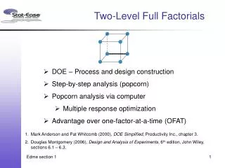
Two-Level Full Factorials
Two-Level Full Factorials. DOE – Process and design construction Step-by-step analysis (popcorn) Popcorn analysis via computer Multiple response optimization Advantage over one-factor-at-a-time (OFAT). Mark Anderson and Pat Whitcomb (2000), DOE Simplified , Productivity Inc., chapter 3.

Two-Level Full Factorials
E N D
Presentation Transcript
Two-Level Full Factorials • DOE – Process and design construction • Step-by-step analysis (popcorn) • Popcorn analysis via computer • Multiple response optimization • Advantage over one-factor-at-a-time (OFAT) • Mark Anderson and Pat Whitcomb (2000), DOE Simplified, Productivity Inc., chapter 3. • Douglas Montgomery (2006), Design and Analysis of Experiments, 6th edition, John Wiley, sections 6.1 – 6.3.
Agenda Transition • DOE – Process and design constructionIntroduce the process for designing factorial experiments and motivate their use. • Step-by-step analysis (popcorn) • Popcorn analysis via computer • Multiple response optimization • Advantage over one-factor-at-a-time (OFAT)
Controllable Factors “x” Process Responses “y” Noise Factors “z” Design of Experiments • DOE (Design of Experiments) is: • “A systematic series of tests, in which purposeful changes are made to input factors, • so that you may identify causes for significant changes in the output responses.”
Iterative Experimentation Conjecture • Expend no more than 25% of budget on the 1st cycle. Analysis Design Experiment
DOE Process (1 of 2) • Identify opportunity and define objective. • State objective in terms of measurable responses. • Define the change (Dy) that is important to detect for each response. • Estimate experimental error (s) for each response. • Use the signal to noise ratio (Dy/s) to estimate power. • Select the input factors to study. (Remember that the factor levels chosen determine the size of Dy.)
DOE Process (2 of 2) • Select a design and: • Evaluate aliases (details in section 4). • Evaluate power (details in section 2). • Examine the design layout to ensure all the factor combinations are safe to run and are likely to result in meaningful information (no disasters). We will begin using and flesh out the DOE Process in the next section.
Controllable Factors “x” Process Responses “y” Noise Factors “z” Design of Experiments Let’s brainstorm. What process might you experiment on for best payback? How will you measure the response? What factors can you control? Write it down.
Central Limit TheoremCompare Averages NOT Individuals • Jacob Bernoulli (1654-1705) • The ‘Father of Uncertainty’ • “Even the most stupid of men, by some instinct of nature, by himself and without any instruction, is convinced that the more observations have been made, the less danger there is of wandering from one’s goal.”
Central Limit TheoremCompare Averages NOT Individuals • As the sample size (n) becomes large, the distribution of averages becomes approximately normal. • The variance of the averages is smaller than the variance of the individuals by a factor of n. s (sigma) symbolizes true standard deviation • The mean of the distribution of averages is the same as the mean of distribution of individuals. (mu) symbolizes true population mean The CLT applies regardless of the distribution of the individuals.
2 6 1 3 4 5 A v e r a g e s o f T w o D i c e _ _ _ 5 6 _ 1 2 _ 4 4 5 6 _ 1 2 3 3 _ 3 3 3 4 6 5 _ 2 3 4 1 4 4 _ 2 2 6 2 2 3 4 5 _ 4 1 2 3 5 5 5 5 _ 1 1 2 1 3 4 5 6 1 1 _ 1 2 3 4 5 6 6 6 6 6 2 6 1 3 4 5 Central Limit TheoremIllustration using Dice • Individuals are uniform; averages tending toward normal! Example: "snakeyes" [1/1] is the only way to get an average of one.
Central Limit TheoremUniform Distribution • As the sample size (n) becomes large, the distribution of averages becomes approximately normal. • The variance of the averages is smaller than the variance of the individuals by a factor of n. • The mean of the distribution of averages is the same as the mean of distribution of individuals.
Motivation for Factorial Design • Want to estimate factor effects well; this implies estimating effects from averages.Refer to the slides on the Central Limit Theorem. • Want to obtain the most information in the fewest number of runs. • Want to estimate each factor effect independent of the existence of other factor effects. • Want to keep it simple.
Two-Level Full Factorial Design • Run all high/low combinations of 2 (or more) factors • Use statistics to identify the critical factors 22 Full Factorial What could be simpler?
Agenda Transition • DOE – Process and design construction • Step-by-step analysis (popcorn)Learn benefits and basics of two-level factorial design by working through a simple example. • Popcorn analysis via computer • Multiple response optimization • Advantage over one-factor-at-a-time (OFAT)
Two Level Factorial DesignAs Easy As Popping Corn! • Kitchen scientists* conducted a 23 factorial experiment on microwave popcorn. The factors are: • A. Brand of popcorn • B. Time in microwave • C. Power setting • A panel of neighborhood kids rated taste from one to ten and weighed the un-popped kernels (UPKs). * For full report, see Mark and Hank Andersons' Applying DOE to Microwave Popcorn, PIQuality 7/93, p30.
Two Level Factorial DesignAs Easy As Popping Corn! * Average scores multiplied by 10 to make the calculations easier.
Two Level Factorial DesignAs Easy As Popping Corn! Factors shown in coded values
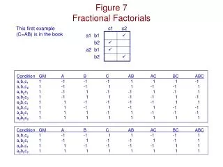
R1 - Popcorn TasteAverage A-Effect There are four comparisons of factor A (Brand), where levels of factors B and C (time and power) are the same: 75 – 74 = + 1 80 – 71 = + 9 77 – 81 = – 4 32 – 42 = – 10
R1 - Popcorn TasteAnalysis Matrix in Standard Order • I for the intercept, i.e., average response. • A, B and C for main effects (ME's). These columns define the runs. • Remainder for factor interactions (FI's)Three 2FI's and One 3FI.
Sparsity of Effects Principle • Do you expect all effects to be significant? • Two types of effects: • Vital Few: • About 20 % of ME's and 2 FI's will be significant. • Trivial Many: • The remainder result from random variation.
Estimating Noise • How are the “trivial many” effects distributed? • Hint: Since the effects are based on averages you can apply the Central Limit Theorem. • Hint: Since the trivial effects estimate noise they should be centered on zero. • How are the “vital few” effects distributed? • No idea! Except that they are too large to be part of the error distribution.
Half Normal Probability PaperSorting the vital few from the trivial many. Significant effects (the vital few) are outliers. They are too big to be explained by noise. They’re "keepers"! Negligible effects (the trivial many) will be N(0, s), so they fall near zero on straight line. These are used to estimate error.
Half Normal Probability PaperSorting the vital few from the trivial many. Significant effects: The model terms! Negligible effects:The error estimate!
Half Normal Probability Paper (taste)Sorting the vital few from the trivial many. • Sort absolute value of effects into ascending order, “i”. Enter C & BC effects. • Compute Pis for effects. Enter Pis for i = 5 & 7. • Label the effects. Enter labels for C & BC effects.
Half Normal Probability Paper (taste)Sorting the vital few from the trivial many.
Analysis of Variance (taste)Sorting the vital few from the trivial many. Compute Sum of Squares for C and BC:
Analysis of Variance (taste)Sorting the vital few from the trivial many. • Add SS for significant effects: B, C & BC. • Call these vital few the “Model”. • Add SS for negligible effects: A, AB, AC & ABC. • Call these trivial many the “Residual”.
Analysis of Variance (taste)Sorting the vital few from the trivial many. F-value = 31.5 0.001 < p-value < 0.005
Analysis of Variance (taste)Sorting the vital few from the trivial many • Null Hypothesis:There are no effects, that is: H0: A= B=…= ABC= 0 • F-value: • If the null hypothesis is true (all effects are zero) then the calculated F-value is 1. • As the model effects (B, C and BC) become large the calculated F-value becomes >> 1. • p-value: • The probability of obtaining the observed F-value or higher when the null hypothesis is true.
Agenda Transition • DOE – Process and design construction • Step-by-step analysis (popcorn) • Popcorn analysis via computerLearn to extract more information from the data. • Multiple response optimization • Advantage over one-factor-at-a-time (OFAT)
Popcorn via Computer! • Use Design-Expert to build and analyze the popcorn DOE:
Popcorn Analysis via Computer!Instructor led(page 1 of 2) • File, New Design. • Build a design for 3 factors, 8 runs. • Enter factors: Leave delta and sigma blank to skip power calculations. Power will be introduced in section 2! • Enter responses.
Popcorn Analysis via Computer!Instructor led(page 2 of 2) • Right-click on Std column header and choose “Sort by Standard Order”. • Type in response data (from previous page) for Taste and UPKs. • Analyze Taste. • Taste will be instructor led; you will analyze the UPKs on your own. • Save this design.
Popcorn Analysis – Taste Effects Button - View, Effects List • Term Stdized Effect SumSqr % Contribution • Require Intercept • Error A-Brand -1 2 0.0819001 • Error B-Time -20.5 840.5 34.4185 • Error C-Power -17 578 23.6691 • Error AB 0.5 0.5 0.020475 • Error AC -6 72 2.9484 • Error BC -21.5 924.5 37.8583 • Error ABC -3.5 24.5 1.00328 • Lenth's ME 33.8783 • Lenth's SME 81.0775
Popcorn Analysis – TasteEffects -View,Half Normal Plot of Effects
Popcorn Analysis – TasteEffects -View,Pareto Chart of “t” Effects
Popcorn Analysis – Taste ANOVA button • Analysis of variance table [Partial sum of squares] • Sum of Mean F • Source Squares df Square Value Prob > F • Model 2343.00 3 781.00 31.56 0.0030 • B-Time 840.50 1 840.50 33.96 0.0043 • C-Power 578.00 1 578.00 23.35 0.0084 • BC 924.50 1 924.50 37.35 0.0036 • Residual 99.00 4 24.75 • Cor Total 2442.00 7
Popcorn Analysis – Taste ANOVA (summary statistics) • Std. Dev. 4.97 R-Squared 0.9595 • Mean 66.50 Adj R-Squared 0.9291 • C.V. % 7.48 Pred R-Squared 0.8378 • PRESS 396.00 Adeq Precision 11.939
Popcorn Analysis – Taste ANOVA Coefficient Estimates • Coefficient Standard 95% CI 95% CI • Factor Estimate DF Error Low High VIF • Intercept 66.50 1 1.76 61.62 71.38 • B-Time -10.25 1 1.76 -15.13 -5.37 1.00 • C-Power -8.50 1 1.76 -13.38 -3.62 1.00 • BC -10.75 1 1.76 -15.63 -5.87 1.00 Coefficient Estimate: One-half of the factorial effect (in coded units)
Popcorn Analysis – Taste Predictive Equation (Coded) Final Equation in Terms of Coded Factors: Taste = +66.50 -10.25*B -8.50*C -10.75*B*C
Popcorn Analysis – Taste Predictive Equation (Actual) Final Equation in Terms of Actual Factors: Taste = -199.00 +65.00*Time +3.62*Power -0.86*Time*Power
Popcorn Analysis – Taste Predictive Equations Coded Factors: Taste =+66.50 -10.25*B -8.50*C -10.75*B*C Actual Factors: Taste =-199.00 +65.00*Time +3.62*Power -0.86*Time*Power • For process understanding, use coded values: • Regression coefficients tell us how the response changes relative to the intercept. The intercept in coded values is in the center of our design. • Units of measure are normalized (removed) by coding. Coefficients measure half the change from –1 to +1 for all factors.
Factorial DesignResidual Analysis Independent N(0,s2)
Popcorn Analysis – Taste Diagnostic Case Statistics • Diagnostics → Influence → Report • Diagnostics Case Statistics • Internally Externally Influence on • Std Actual Predicted Studentized Studentized Fitted Value Cook's Run • Order Value Value Residual Leverage Residual Residual DFFITS Distance Order • 1 74.00 74.50 -0.50 0.500 -0.142 -0.123 -0.123 0.005 8 • 2 75.00 74.50 0.50 0.500 0.142 0.123 0.123 0.005 1 • 3 71.00 75.50 -4.50 0.500 -1.279 -1.441 -1.441 0.409 2 • 4 80.00 75.50 4.50 0.500 1.279 1.441 1.441 0.409 4 • 5 81.00 79.00 2.00 0.500 0.569 0.514 0.514 0.081 3 • 6 77.00 79.00 -2.00 0.500 -0.569 -0.514 -0.514 0.081 5 • 7 42.00 37.00 5.00 0.500 1.421 1.750 1.750 0.505 7 • 8 32.00 37.00 -5.00 0.500 -1.421 -1.750 -1.750 0.505 6 See “Diagnostics Report – Formulas & Definitions” in your “Handbook for Experimenters”.
Factorial DesignANOVA Assumptions • Additive treatment effects • Factorial: An interaction model will adequately represent response behavior. • Independence of errors • Knowing the residual from one experiment givesno information about the residual from the next. • Studentized residuals N(0,s2): • Normally distributed • Mean of zero • Constant variance, s2=1 • Check assumptions by plotting studentized residuals! • Model F-test • Lack-of-Fit • Box-Cox plot S ResidualsversusRun Order Normal Plot ofS Residuals S ResidualsversusPredicted