Active Contours - SNAKES
CSci 8810 Image Processing. Active Contours - SNAKES. Meghana Viswanath March 19, 2009. Object Recognition… How?. Edge detectors. Works well for some images. Not so much for others. Too many spurious edges Linking edges belonging to the same object is difficult. Active Contours or Snakes.

Active Contours - SNAKES
E N D
Presentation Transcript
CSci 8810 Image Processing Active Contours - SNAKES Meghana Viswanath March 19, 2009
Object Recognition… How? • Edge detectors Works well for some images
Not so much for others • Too many spurious edges • Linking edges belonging to the same object is difficult
Active Contours or Snakes • Results from the work of Kass et.al. in 1987 • Snakes are shapes or curves that transform themselves to take the shape of an object in an image. • Snakes are energy minimizing splines
Snake Behavior • An initial curve/snake is defined near the object • The curve is iteratively refined to form the least energy contour • Snakes operate locally, thus one must provide an initial position for them
Snake Representation • A snake is a contour in the image plane, defined by a set of ncontrol points. vi = (xi, yi), i = 0, .... n-1
Energy Minimization vi-1 vi vi+1 snake object boundary Find the local minimum and move towards it.
Snake Energy The snake - v(s) = [x(s), y(s)], is defined as a function of a real variable s ϵ [0,1] The energy of the snake is given by - Esnake = 0∫1 (Eint + Eext)ds
Internal Energy • Internal energy describes the manner in which the snake moves • It can be written as - Eint = (α (v’)2 + β (v”)2) • α, β specify the amount of elasticity and stiffness of the snake, respectively
Internal Energy • First Term : α (v’)2 • If you want the snake to shrink, then make Eint directly proportional to snake length • Instead, Eint = Σα (distance b/w control pt. and left neighbour)2 • This makes the control points to spread out evenly
Internal Energy • Second Term : β (v”)2 • If you want the snake to be smooth, then make Eint directly proportional to the curvature • Instead, Eint = Σβ (curvature at control point)2 • This makes the control points to move as a smooth curve
Internal Energy • A large positive value of α and/or β means that stretching(elasticity) and/or bending(smoothness) are tightly constrained as we search for an energy minimum • Making β = 0 i.e. second order discontinuous, makes the snake develop a corner (least stiff)
External Energy • External energy pulls the snake towards desirable features such as edges • Tells the snake where to stop • It is derived from the image • External energy – negative gradient Eext = -|∇I(x,y)|2
For a gray-scale image I(x,y), Eext = -|∇ I(x,y)|2 Eext = -|∇ (Gσ(x,y) * I(x,y))|2 For a binary image Eext = I(x,y) Eext = Gσ(x,y) * I(x,y) External Energy
Euler Equation • A snake that minimizes E must satisfy the Euler equation – α v”(s)- β v””(s) -∇Eext = 0
Force Balance Equation Minimizing energy equation can be interpreted as a force balance equation Fint + Fext = 0 where Fint = α v” - β v”” and Fext = −∇ Eext The internal force Fint discourages stretching and bending while the external potential force Fext pulls the snake toward the desired image edges
Problems with traditional snakes • Low capture range • Initial snake position should be close to the object boundary • Reason - External force field is non-existent in uniform regions • Unable to move into boundary concavities • Reason – External force vectors are normal to the object boundary
Traditional Snakes (a) (a) (a) (b) (b) (b) (c) (c) • Convergence of the snake • External Force Field • Close-up of the force field within the boundary concavity
Gradient Vector Flow (GVF) snakes Both problems with traditional snakes are related to external force field. Xu and Prince formulate a new type of static external force called Gradient Vector Flow. Fext = v
Edge Map • For any gray-scale or binary image, let the edge map be defined such that it has large values near edges. Eg.Eext =-|∇ I(x,y)|2 • Properties of edge maps • Gradient vectors point toward and are normal to the edges • Gradients are large only in the immediate neighborhood of edges • In homogeneous regions, gradient is almost zero
How edge map properties affect traditional snake behavior • Gradient vectors point toward and are normal to the edges => a snake initialized close to the edge will converge to a stable configuration near the edge • Gradients are large only in the immediate neighborhood of edges => small capture range • In homogeneous regions, gradient is almost zero => homogeneous regions will have no external forces
GVF Approach • Retain the highly desirable property of the gradients near the edges • But extend the gradient map farther away from the edges and into homogeneous regions using a computational diffusion process. • As an important benefit, the inherent competition of the diffusion process will also create vectors that point into boundary concavities.
GVF energy functional • We define the gradient vector flow field to be the vector fieldv(x,y)=(u(x,y),v(x,y)) that minimizes the energy functional Ɛ = ∫ ∫ Ч(ux2+uy2+vx2+vy2)+|∇ f |2|v-∇ f |2dxdy • When ∇ f is low, the first term dominates yielding a slowly varying field • When ∇ f is high, the second term dominates and is minimized by setting v =∇ f.
GVF Euler equations • It can be shown that the GVF field can be found by solving the following Euler equations – • In homogeneous regions, second term = 0 • u and v are determined only by the Laplace equation • v is determined from the region’s boundary • a kind if competition among boundary vectors Therefore, GVF snakes can move into boundary concavities
GVF Snakes (a) (b) (c) • Convergence of the snake • External Force Field • Close-up of the force field within the boundary concavity
Applications • Motion Tracking • Speech Analysis • Traffic monitoring • Surveillance • Actor-driven facial animation • Gait Analysis
Traffic Monitoring By automatically tracking cars, the emergency services could obtain rapid warning of an accident or traffic jam.
Surveillance A computer vision system follows an intruder on a security camera
Actor-driven facial animation Tracked facial motions drive input channels to a cartoon cat, programmed with some exaggeration of expression
Motion Tracking Tracking the articulated motion of a human body is applicable both to biometrics and clinical gait analysis and for actor-driven whole body animation
References Books - • Computer Vision – L. Shapiro and G. Stockman • Active Contours – Blake and Isard Technical papers - • Snakes: Active contour models - M. Kass, A. Witkin and D. Terzopoulos. • Snakes, Shapes, and Gradient Vector Flow - Chenyang Xu and Jerry L. Prince