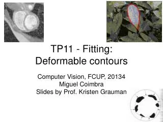
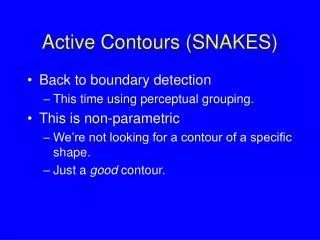
Active Contours (SNAKES)
Active Contours (SNAKES). Back to boundary detection This time using perceptual grouping. This is non-parametric We’re not looking for a contour of a specific shape. Just a good contour. For Information on SNAKEs. Not in Forsyth and Ponce.

Active Contours (SNAKES)
E N D
Presentation Transcript
Active Contours (SNAKES) • Back to boundary detection • This time using perceptual grouping. • This is non-parametric • We’re not looking for a contour of a specific shape. • Just a good contour.
For Information on SNAKEs • Not in Forsyth and Ponce. • See Text by Trucco and Verri, or Shapiro and Stockman. • Kass, Witkin and Terzopoulos, IJCV. • “Dynamic Programming for Detecting, Tracking, and Matching Deformable Contours”, by Geiger, Gupta, Costa, and Vlontzos, IEEE Trans. PAMI 17(3)294-302, 1995 • E. N. Mortensen and W. A. Barrett, Intelligent Scissors for Image Composition, in ACM Computer Graphics (SIGGRAPH `95), pp. 191-198, 1995
Improve Boundary Detection • Integrate information over distance. • Use Gestalt cues • Smoothness • Closure • Get User to Help.
Strategy of Class • What is a good path? • Given endpoints, how do we find a good path? • What if we don’t know the end points? Note that like all vision this is modeling and optimization.
We’ll do something easier than finding the whole boundary. Finding the best path between two boundary points.
How do we decide how good a path is? Which of two paths is better?
Discrete Grid • Contour should be near edge. • Strength of gradient. • Contour should be smooth (good continuation). • Low curvature • Low change of direction of gradient.
Review Gradient Blackboard: See notes on Class 6 also.
Smoothness • Discrete Curvature: if you go from p(j-1) to p(j) to p(j+1) how much did direction change? • Be careful with discrete distances. • Change of direction of gradient from p(j-1) to p(j)
Combine into a cost function • Path: p(1), p(2), … p(n). • Where • d(p(j),p(j+1)) is distance between consecutive grid points (ie, 1 or sqrt(2). • g(p(j)) measures strength of gradient • l is some parameter • f measures smoothness, curvature.
One Example cost function f is the angle between the gradient at p(j-1) and p(j). Or it could more directly measure curvature of the curve. (Loosely based on “Dynamic Programming for Detecting, Tracking, and Matching Deformable Contours”, by Geiger, Gupta, Costa, and Vlontzos, IEEE Trans. PAMI 17(3)294-302, 1995.)
So How do we find the best Path? Computer Science at last. A Curve is a path through the grid. Cost depends on each step of the path. We want to minimize cost.
Map problem to Graph Weight represents cost of going from one pixel to another. Next term in sum.
9 4 5 1 3 3 3 2 Dijkstra’s shortest path algorithm link cost 0 • Algorithm • init node costs to , set p = seed point, cost(p) = 0 • expand p as follows: for each of p’s neighbors q that are not expanded • set cost(q) = min( cost(p) + cpq, cost(q) ) (Seitz)
9 4 5 1 3 3 3 2 Dijkstra’s shortest path algorithm 4 9 5 1 1 1 0 3 3 2 3 • Algorithm • init node costs to , set p = seed point, cost(p) = 0 • expand p as follows: for each of p’s neighbors q that are not expanded • set cost(q) = min( cost(p) + cpq, cost(q) ) • if q’s cost changed, make q point back to p • put q on the ACTIVE list (if not already there)
9 4 5 1 3 3 3 2 Dijkstra’s shortest path algorithm 4 9 5 2 3 5 2 1 1 0 3 3 3 4 3 2 3 • Algorithm • init node costs to , set p = seed point, cost(p) = 0 • expand p as follows: for each of p’s neighbors q that are not expanded • set cost(q) = min( cost(p) + cpq, cost(q) ) • if q’s cost changed, make q point back to p • put q on the ACTIVE list (if not already there) • set r = node with minimum cost on the ACTIVE list • repeat Step 2 for p = r
9 4 5 1 3 3 3 2 Dijkstra’s shortest path algorithm 4 3 6 5 2 3 5 3 2 1 1 0 3 3 3 4 4 3 2 2 3 • Algorithm • init node costs to , set p = seed point, cost(p) = 0 • expand p as follows: for each of p’s neighbors q that are not expanded • set cost(q) = min( cost(p) + cpq, cost(q) ) • if q’s cost changed, make q point back to p • put q on the ACTIVE list (if not already there) • set r = node with minimum cost on the ACTIVE list • repeat Step 2 for p = r
Results (Seitz Class) demo
Continuous versions • Can express cost function as continuous. • Use continuous optimization like gradient descent. • Level Set methods. • These lead to local optima near a starting point.
Why do we need user help? • Why not run all points shortest path and find best closed curve?
Lessons • Perceptual organization, middle level knowledge, needed for boundary detection. • Fully automatic methods not good enough yet. • Formulate desired solution then optimize it.