CONTOURS
CONTOURS. BY, Jayesh Raghavan Electrical Engineering Department The University of Texas at Arlington. OVERVIEW. GEOMETRY OF CURVES CONTOUR PROPERTIES CURVE FITING. CONTOUR. Edges : - Significant local changes in image, occur on the boundary between 2 different regions in an image.


CONTOURS
E N D
Presentation Transcript
CONTOURS BY, JayeshRaghavan Electrical Engineering Department The University of Texas at Arlington. Computer Vision
OVERVIEW GEOMETRY OF CURVES CONTOUR PROPERTIES CURVE FITING Computer Vision
CONTOUR Edges : - Significant local changes in image, occur on the boundary between 2 different regions in an image. Edges are linked into a representation for a region boundary called contour. The contours correspond to region boundaries. Computer Vision
CONTOUR (contd….) • Can be classified in two ways :- Closed Contour :- - Correspond to a region boundaries. Open Contour :- - Part of a region boundary. Computer Vision
BIT MORE ON CONTOUR • A contour is a sequence of 8 – connected pixels in an image where each pixel can be reached from any other pixel in the contour. • An open contour has two end pixels each with only one neighbor, and zero or more interior pixels, each with exactly two neighbors. • A closed contour has no end pixels. All pixels in a closed contour have exactly two neighbor Computer Vision
BIT MORE ON CONTOUR • The length of a contour is computed from the sum of distances between adjacent pixels in the contour. • Two adjacent pixels that lie horizontally or vertically are considered to be apart by 1 pixel. All other adjacent pixels are considered to be apart by 2 pixels. Computer Vision
CRITERIA TO REPRESENT A GOOD CONTOUR • Efficiency – Simple, compact representation. • Accuracy – Fit images features accurately. • Effectiveness – Suitable for the operation performed in the later stages of the application. • Accuracy of estimating of edge locations. • Performance of the curve fitting algorithm. Computer Vision
WAYS OF REPRESENTING A CONTOUR • Ordered List:- The simplest representation of contour. • Efficiency – Least compact & simplest. • Accuracy – Depends on how accurately edge locations are estimated. • Curves:- The most powerful representation as it involves fitting a curve having some analytical description ( Polygonal – curves, lines segments etc…) • More compact. • Efficient and Accurate. Computer Vision
-- FEW DEFINITIONS -- • An Edge list is an ordered set of edge points. • A contour is an edge list or the curve that has been used to represent the edge list. • A boundary is the closed contour that surrounds a region. • A curve interpolates a list of points if it passes through the points. • A curve approximates a list of points if it passes close to the edge points, but not necessarily passing exactly through them. Computer Vision
INTERPOLATION Vs APPROXIMATION Computer Vision
INTERPOLATION Vs APPROXIMATION • A curve interpolates a list of points if it passes through the points. • A curve approximates a list of points if it passes close to the points, but not necessarily passing exactly through the points. • Curve interpolation methods are more appropriate when the edges have been extracted accurately. • In practice, curve approximation methods yield better results because the edge locations can not be extracted very accurately. Computer Vision
GEOMETRY OF CURVES1.Representing a point - Explicit form y = f(x) - Implicit form f(x,y)=0 - Parametric form (x(u), y(u))u is the parameter2.Length of an arc Computer Vision
DIGITAL CONTOURS • The length of a digital contour p1 = (x1, y1), p2 = (x2, y2), ..., pi = (xi, yi) can be approximated by adding the lengths of the individual segments between edge points: • Distance between end points can be calculated as: Computer Vision
DIGITAL CONTOURS • Slope (tangent) and curvature are difficult to compute precisely since the angle between neighboring edge pixels is quantized to 45 degrees increments. • The idea is to compute the slope using edge points that are not adjacent: - left k-slope: the direction between points pi-k and pi - right k-slope: the direction between points pk and pi+k - k-curvature: the difference between the left and right k-slopes. Computer Vision
SIMPLE METHODS • Chain Codes • Crack Codes • Slope Representation • Slope Density Function • Centroidal Profile Representation Computer Vision
CHAIN CODES • Chain-code representation Specifies the direction of each edge point along the contour. • Start at the first edge point and go clockwise around the contour. • The direction to the next edge point is specified using one of the four or eight quantized directions. Computer Vision
CHAIN CODES Computer Vision
CHAIN CODES chain code: 0033333...01 Computer Vision
LIMITATIONS OF CHAIN CODES • Chain code of a boundary depends on the starting point. • Limited set of directions. • Sensitive to noise Computer Vision
CRACK CODES • An alternative to the chain code for contour encoding is to use neither the contour pixels associated with the object nor the contour pixels associated with background but rather the line, the "crack", in between them. • Directions are quantized into 4 directions. Computer Vision
SLOPE REPRESENTATION • Its an continuous version of chain code. • Start at the first edge point and go clockwise around the contour. • Estimate the slope(y) and arc length(s) using the formulas given previously for digital contours. • Plot the slope versus the arc-length. Computer Vision
SLOPE REPRESENTATION 4) Horizontal line in the y-s space correspond to segments in the contour . 5) Line segments at the other orientations correspond to circular arcs. 6) Portions of the plot that are not straight line segments correspond to other curve primitives. Computer Vision
SLOPE REPRESENTATION Computer Vision
FEW COMMENTS • Different starting points cause a shift in the s-axis. • Rotations cause a shift in the Ψ axis. • Not very tolerant to noise. • For a closed contour this plot is periodic. Computer Vision
SLOPE DENSITY FUNCTION • Histogram of the slopes along the contour. • Orientation can be determined using correlation of slope histograms. • Can be very useful for object recognition. Computer Vision
90 180 0 Density Density Density Density 270 Square Diamond 0 0 0 0 90 90 90 90 180 180 180 180 270 270 270 270 360 360 360 360 Angle Angle Angle Angle Circle Ellipse EXAMPLES Computer Vision
CENTROIDAL PROFILE REPRESENTATION Plot the distance from the centroid to the boundary as a function of angle. Computer Vision
CONTOUR REPRESENTATION USING CURVE FITTING (INTERPOLATION) • The main assumption when using interpolation is that the edge points have been extracted accurately. • Errors in edge locations can be handled better using curve-fitting based on approximation. Computer Vision
EVALUATING THE GOODNESS OF THE FIT • Maximum absolute error: measures how much the points deviate from the curve in the worst case. MAE = maxi |di | • Mean squared error: gives an overall measure of the deviation of the curve from the edge points. Computer Vision
EVALUATING THE GOODNESS OF THE FIT • Normalized maximum absolute error: the ratio of the maximum absolute error to the length of the curve (error becomes independent of the length of the curve). NMAE = maxi |di |/L • Ration of curve length to the end point distance: a good measure of the complexity of the curve. Computer Vision
POLYLINE REPRESENTATION A polyline is a sequence of line segments joined end to end. The ends of each line are edge points in the original edge list. The points where line segments are joined are called vertices. Computer Vision
DISTANCE OF POINT FROM LINE • Equation of line passing from two points (x1, y1), (x2, y2): x(y1 - y2) + y(x1 - x2) + y2 x1 - y1 x2 = 0 • Distance d of edge point (u, v) from the line: d =r/D • r=u(y1 - y2) + v(x1 - x2) + y2 x1 - y1 x2 • D is the distance between (x1, y1) and (x2, y2). Computer Vision
CURVE FITTING MODELS • Straight line segments • Circular arcs • Conic sections • Cubic splines Computer Vision
POLYLINE REPRESENTATION TYPES • Splitting • Merging • Split and Merge Algorithm • Hop-Along Algorithm Computer Vision
SPLIT ALGORITHM(top-down) • Take the line segment connecting the end points of the contour (if the contour is closed, consider the line segment connecting the two farthest points). • Find the farthest edge point from the line segment. • If the normalized maximum error of that point from the line segment is above a threshold, split the segment into two segments at that point (i.e., new vertex). • Repeat the same procedure for each of the two sub segments until the error is very small. Computer Vision
EXAMPLE (Open Contour) Computer Vision
EXAMPLE (Closed Contour) Computer Vision
MERGE ALGORITHM (Bottom-Up) • Use the first two edge points to define a line segment. • Add a new edge point if it does not deviate too far from the current line segment. • Update the parameters of the line segment using least-squares. • Start a new line segment when edge points deviate too far from the line segment. Computer Vision
EXAMPLE Computer Vision
SPLIT AND MERGE ALGORITHM • The accuracy of line segment approximations can be improved by interleaving merge and split operations. • After recursive subdivision (split), allow adjacent segments to be replaced by a single segment (merge). • Alternate applications of split and merge until no segments are merged or split. Computer Vision
EXAMPLE Computer Vision
HOP – ALONG ALGORITHM • Start with the first k edges from the list. • Fit a line segment between the first and the last edges in the sub list. • If the normalized maximum error is too large, shorten the sub list sub list to the point of maximum error. Return to step 2. • If the line fit succeeds, compare the orientation of the current line segment with that of the previous line segment. If the lines have similar orientations, replace the two line segments with a single line segment. Computer Vision
HOP – ALONG ALGORITHM • Make the current line segment the previous line segment and advance the window of edges so that there are k edges in the sub list. Return to step 2. Computer Vision
CIRCULAR ARCS • Once an edge list has been approximated by line segments, subsequences of the line segments can be replaced by circular arcs. • This involves fitting circular arcs through the endpoints of two or more line segments. Computer Vision
CIRCULAR ARCS (ALGO….) • Initialize the window of vertices to the three endpoints of the first two line segments in the polygonal approximation. • Compute the ratio of the length of the part of the contour corresponding to the two line segments to the distance between the end points. If the ratio is small, then leave the first line segment unchanged, advance the window of vertices by one vertex, and repeat this step. • Fit a circle through the three vertices. Computer Vision
CIRCULAR ARCS (ALGO…..) 4. If the fit is not good (i.e., normalized maximum error is too large), then leave the first line segment unchanged, advance the window of vertices, and return to step 2. 5. If the circle fit succeeds, then try to include the next line segment in the circular arc. Repeat this step until no more line segments can be subsumed by this circular arc. 6. Advance the window to the next three polygon vertices after the end of the circular arc and return to step 2. Computer Vision
CONIC SECTIONS AND CUBIC SPLINES • Conic sections correspond to hyperbolas, parabolas, and ellipses (2nd degree polynomials). • Cubic splines correspond to 3rd degree polynomials. • Conic sections and cubic splines allow more complex contours to be represented using fewer segments. Computer Vision
CONTOUR REPRESENTATION USING CURVE FITTING • Higher accuracy can be obtained by computing an approximation that is not forced to pass through particular edge points. • Approximation-based methods use all the edge points to find a good fit (this is contrast to the previous methods that use only the interpolated edge points). • Methods to approximate curves depend on the reliability with which edge points can be grouped into contours. (1) Least-squares regression can be used if it is certain that the edge points grouped together belong to the same contour. (2) Robust regression is more appropriate if there are some grouping errors. Computer Vision
LEAST – SQUARES LINE FIT • Linear regression fits a line to the edge points by minimizing the sum of squares of the perpendicular distances of the edge points from the line being fit. Computer Vision
The solution to the linear regression problem is:- where, Computer Vision