Download

1 / 38
390 likes | 615 Vues
Analysis and Design of Asynchronous Transfer Lines as a series of G/G/m queues. Topics. The negative impact of variability in the operation of Asynchronous Transfer Lines Modeling the Asynchronous Transfer Line as a series of G/G/m queues Modeling the impact of various operational detractors

E N D
Analysis and Design of Asynchronous Transfer Lines as a series of G/G/m queues
Topics • The negative impact of variability in the operation of Asynchronous Transfer Lines • Modeling the Asynchronous Transfer Line as a series of G/G/m queues • Modeling the impact of various operational detractors • Employing the derived models in line diagnosis • Employing the derived models in line design
W1 TH TH B1 M1 Asynchronous Transfer Lines (ATL) W2 W3 TH TH B2 M2 B3 M3 • Some important issues: • What is the maximum throughput that is sustainable through this line? • What is the expected cycle time through the line? • What is the expected WIP at the different stations of the line? • What is the expected utilization of the different machines? • How does the adopted batch size affect the performance of the line? • How do different detractors, like machine breakdowns, setups, and maintenance, affect the performance of the line?
TH B1 M1 Analyzing a single workstation with deterministic inter-arrival and processing times Case I: ta = tp = 1.0 WIP 1 TH = 1 part / time unit Expected CT = tp t 1 2 3 4 5 Arrival Departure
TH B1 M1 Analyzing a single workstation with deterministic inter-arrival and processing times Case II: tp = 1.0; ta = 1.5 > tp WIP Starvation! 1 TH = 2/3 part / time unit Expected CT = tp t 1 2 4 5 3 Arrival Departure
TH B1 M1 3 2 1 t 1 2 3 4 5 Arrival Departure Analyzing a single workstation with deterministic inter-arrival and processing times Case III: tp = 1.0; ta = 0.5 WIP Congestion! TH = 1 part / time unit Expected CT
TH B1 M1 A single workstation with variable inter-arrival times Case I: tp=1; taN(1,0.12) (ca=a / ta = 0.1) WIP 3 2 TH < 1 part / time unit Expected CT 1 t 1 2 3 4 5 Arrival Departure
TH B1 M1 WIP 3 2 1 t 1 2 3 4 5 Arrival Departure A single workstation with variable inter-arrival times Case II: tp=1; taN(1,1.02) (ca=a / ta = 1.0) TH < 1 part / time unit Expected CT
TH B1 M1 WIP 3 2 1 t 1 2 3 4 5 A single workstation with variable processing times Case I: ta=1; tpN(1,1.02) TH < 1 part / time unit Expected CT Arrival Departure
Remarks • Synchronization of job arrivals and completions maximizes throughput and minimizes experienced cycle times. • Variability in job inter-arrival or processing times causes starvation and congestion, which respectively reduce the station throughput and increase the job cycle times. • In general, the higher the variability in the inter-arrival and/or processing times, the more intense its disruptive effects on the performance of the station. • The coefficient of variation (CV) defines a natural measure of the variability in a certain random variable.
TH B1 M1 B2 M2 WIP 3 2 1 t 1 2 3 4 5 The propagation of variability W1 W2 Case I: tp=1; taN(1,1.02) Case II: ta=1; tpN(1,1.02) WIP 3 2 1 t 1 2 3 4 5 W1 arrivals W1 departures W2 arrivals
Remarks • The variability experienced at a certain station propagates to the downstream part of the line due to the fact that the arrivals at a downstream station are determined by the departures of its neighboring upstream station. • The intensity of the propagated variability is modulated by the utilization of the station under consideration. • In general, a highly utilized station propagates the variability experienced in the job processing times, but attenuates the variability experienced in the job inter-arrival times. • A station with very low utilization has the opposite effects.
TH B1 M1 The G/G/1 model:A single-station • Modeling Assumptions: • Part release rate = Target throughput rate = TH • Infinite Buffering Capacity • one server • Server mean processing time = te • St. deviation of processing time = e • Coefficient of variation (CV) of processing time: ce = e / te • Coefficient of variation of inter-arrival times = ca
TH B1 M1 An Important Stability Condition • Average workload brought to station per unit time: • TH·te • It must hold: • Otherwise, an infinite amount of WIP will pile up in front of the station.
TH B1 M1 Performance measures for a stable G/G/1 station • Server utilization: • Expected cycle time in the buffer: (Kingman’s approx.) • Expected cycle time in the station: • Average WIP in the buffer: (by Little’s law) • Average WIP in the station: • Squared CV of the inter-departure times:
Remarks • For a station with variable job inter-arrival and/or processing times, utilization must be strictly less than one in order to attain stable operation. • Furthermore, expected cycle times and WIP grow to very large values as u1.0. • Expected cycle times and WIP can also grow large due to high values of caand/or ce; i.e., extensive variability in the job inter-arrival and/or processing times has a negative impact on the performance of the line. • In case that the job inter-arrival times are exponentially distributed, ca=1.0, and the resulting expression for CTqis exact (a result known as the Pollaczek-Kintchine formula). • The expression for cd2characterizes the propagation of the station variability to the downstream part of the line, and it quantifies the dependence of this propagation upon the station utilization.
M1 TH B TH M2 Mm Performance measures for a stable G/G/m station • Server utilization: • Expected cycle time in the buffer: • Expected cycle time in the station: • Average WIP in the buffer: • Average WIP in the station: • Squared CV of the inter-departure times:
Analyzing a multi-station ATL TH • Key observations: • A target production rate TH is achievable only if each station satisfies the stability requirement u < 1.0. • For a stable system, the average production rate of every station will be equal to TH. • For every pair of stations, the inter-departure times of the first constitute the inter-arrival times of the second. • Then, the entire line can be evaluated on a station by station basis, working from the first station to the last, and using the equations for the basic G/G/m model.
Operational detractors:A primal source for the line variability • Effective processing time = time that the part occupies the server • Effective processing time = Actual processing time + any additional non-processing time • Actual processing time typically presents fairly low variability ( SCV < 1.0). • Non-processing time is due to detractors like machine breakdowns, setups, operator unavailability, lack of consumables, etc. • Detractors are distinguished to preemptive and non-preemptive. Each of these categories requires a different analytical treatment.
Preemptive operational detractors • Outages that take place while the part is being processed. • Some typical examples: • machine breakdowns • lack of consumables • operator unavailability
Modeling the impact of preemptive detractors • X = random variable modeling the natural processing time, following a general distribution. • to = E[X]; o2=Var[X]; co=o / to . • T = random variable modeling the effective processing time = where • Ui= random variable modeling the duration of the i-th outage, following a general distribution, and • N = random variable modeling the number of outages during a the processing of a single part. • mr=E[Ui]; r2=Var[Ui]; cr = r / mr • Time between outages is exponentially distributed with mean mf. • AvailabilityA = mf / (mf+mr) = percentage of time the system is up. • Then, te = E[T] = to / A or equivalently re = 1/te = A (1/to) = A ro
Breakdown Example • Data: Injection molding machine has: • 15 second stroke (to = 15 sec) • 1 second standard deviation (so = 1 sec) • 8 hour mean time to failure (mf = 28800 sec) • 1 hour repair time (mr = 3600 sec) • Natural variabilityco = 1/15 = 0.067 (which is very low)
Example Continued • Effective variability: Which is very high!
Example Continued • Suppose through a preventive maintenance program, we can reduce mf to 8 min and mr to 1 min (the same as before) Which is low!
Non-preemptive operational detractors • Activities that may take place between the processing of two consecutive parts. • Some typical examples: • setups • preventive maintenance • operator breaks
Modeling the impact of non-preemptive detractors • X = random variable modeling the natural processing time, following a general distribution. • to = E[X]; o2=Var[X]; co=o / to . • NS = average number of parts processed between two consecutive setups • It is also assumed that the number of parts between two consecutive setups follows a geometric distribution, which when combined with the previous bullet, it implies that probability for a setup after any given job = 1/ NS. • Z = random variable modeling the duration of a setup • tS = E[Z]; S2 = Var[Z] • S = random variable modeling the setup time experienced by any given job = • T = random variable modeling the effective processing time = X+S • Then, E[S] = tS / NS ; Var[S] = (S2 / NS) + tS2((NS-1) / NS2); te = E[T] = to+tS / NS ; ;
Setup Example • Data: • Fast, inflexible machine: (2 hr setup every 10 jobs) • Slower, flexible machine: (no setups) No difference!
Setup Example (cont.) • Compare mean and variance • Fast, inflexible machine – 2 hr setup every 10 jobs • Slower, flexible machine – no setups • Conclusion: Flexibility can reduce variability.
Setup Example (cont.) • New Machine: Consider a third machine same as previous machine with setups, but with shorter, more frequent setups • Analysis: • Conclusion: Shorter, more frequent setups induce less variability.
M1 B M2 to1=19 min co12=0.25 mf1=48 hrs mr1=8 hrs MTTR ~ expon. to2=22 min co22=1.0 mf2=3.3 hrs mr2=10 min MTTR ~ expon. 20 parts Ca2=1.0 Example:employing the developed theory for diagnostic purposes Desired throughput is TH = 2.4 jobs / hr but practical experience has shown that it is not attainable by this line. We need to understand why this is not possible.
Diagnostics example continued:Capacity analysis based on mean values
Diagnostics example continued:An analysis based on the G/G/m model i.e., the long outages of M1, combined with the inadequate capacity of the interconnecting buffer, starve the bottleneck!
Example: ATL Design • Need to design a new 4-station assembly line for circuit board assembly. • The technology options for the four stations are tabulated below (each option defines the processing rate in pieces per hour, the CV of the effective processing time, and the cost per equipment unit in thousands of dollars).
Example: ATL Design (cont.) • Each station can employ only one technology option. • The maximum production rate to be supported by the line is 1000 panels / day. • The desired average cycle time through the line is one day. • One day is equivalent to an 8-hour shift. • Workpieces will go through the line in totes of 50 panels each, which will be released into the line at a constant rate determined by the target production rate.
A baseline design:Meeting the desired prod. rate with a low cost
Reducing the line cycle time by adding capacity to Station 2
An alternative option:Employ less variable machines at Station 1 This option is dominated by the previous one since it presents a higher CT and also a higher deployment cost. However, final selection(s) must be assessed and validated through simulation.