Waiting Lines Queues
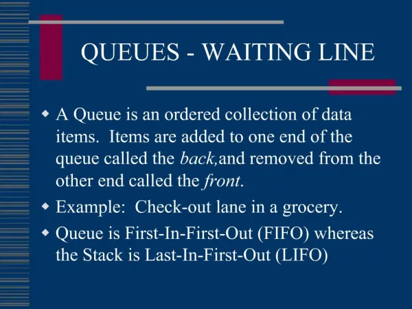
Waiting Lines Queues. Queuing Theory. Managers use queuing models to be more efficient in providing customer service. Models measure average waiting times and average length of waiting lines. Historical Roots.

Waiting Lines Queues
E N D
Presentation Transcript
Queuing Theory • Managers use queuing models to be more efficient in providing customer service. • Models measure average waiting times and average length of waiting lines.
Historical Roots • Agner Krarup Erlang, a Danish engineer who worked for the Copenhagen Telephone Exchange, published the first paper on queueing theory in 1909. • David G. Kendall introduced an A/B/C queueing notation in 1953.
Three queuing disciplines used in Telephone Networks • First In First Out – This principle states that customers are served one at a time and that the customer that has been waiting the longest is served first.[5] • Last In First Out – This principle also serves customers one at a time, however the customer with the shortest waiting time will be served first.[5] • Processor Sharing – Customers are served equally. Network capacity is shared between customers and they all effectively experience the same delay Source: Wikipedia.org
LIFO“Last in First Out” Elevators are a circumstance where this occurs.
Single-server Single-stage Queue Customers In queue Service Facility Arrival Stream Waiting for the Newest ????????
Customers In queue Service Facilities Multiple-server Single-stage Queue
Customers In queue Service Facility Single-server Multiple-stage Queue Pharmacy Conveyor System >>>>>
Multiple-server Multiple-Stage Queue Customers In queue Service Facilities
Little's Theorem • Little's theorem: L = / • The average number of customers (N) can be determined from the following equation: • Here lambda () is the average customer arrival rate and mu () is the average service time for a customer.
Queuing system state probabilities(Basic Model) P0 = 1 - n ( ) Probability distribution for the number of customers in the system = Pn = P0 1, 2, 3,… n =
Queuing Formulas(Basic Model) Average # of Customers in the system L = - 1 L Average Customer Time spent in the system W = = - 2 = Average # of Customers waiting (length of line) Lq ( - ) Lq = Average Customers waiting time Wq= ( - ) = Server Utilization Factor
Phlebotomy Room Example • A queuing system for blood draws. • An average of 25 patients arrive for a blood draw each hour. • One full-time (very experienced) phlebotomist can take one patient every two minutes, thus 30 draws per hour can be done.
Queuing Formulas(Basic Model) = 25 Pts per hour = 30 Pts per hour 25 Average # of Patients in the system: = = 5 customers L = - 30 - 25 1 1 1 Average Patient Time spent in the system: hour = W = = - 5 30 - 25 1 2 (25)2 25 Average # of Patients waiting: 4 = = Lq = = customers 6 30 (30 - 25) ( - ) 6 Lq 25 1 Average Patients waiting time: = hour Wq = = = 30 (30 - 25) 6 ( - ) 25 5 Server Utilization Factor: = = = 30 6 = The phlebotomist is busy five-sixths of the time.
The system state probabilities 25 P0 = 1 - = 1 - = .1667 30 1 25 ( ) ( ) P1 = P0 = (.1667) = .1389 30 2 2 25 ( ) ( ) P2 = P0 = (.1667) = .1158 30 This formula provides the probability that n (0, 1, 2, 3, …) patients will be in the blood drawing room. If you add the individual probabilities for values of n cumulatively you would find 54 in the number of patients where all probabilities of n total 1.
Multiple server models • Uses same notation as basic model but different formulas. • Formulas are based on FIFO discipline. • The customer at the head to waiting line proceeds to the first server. • S = Number of service channels
Queuing system state probabilities(Multiple Servers) ( /)s 1 ( /)n ( ) [ S-1 P0 = 1 + 1 - /S S! n! n=0 ( /)n P0 If 0 < n < S n! Pn = ( /)n If n > S S!Sn-s
Phlebotomy Room Examplewith a second PhlebotomistMultiple Servers • A 2 service channel queuing system for blood draws. • An average of 50 patients arrive for a blood draw each hour. • Two full-time phlebotomists can take one patient each every two minutes, thus 60 draws per hour can be done.
The Probability that there are no patients in the system. S = 2 service channels = 50 Pts per hour = 60 Pts per hour [ 1 ] ( /)0 ( /)1 ( /)2 ( ) P0 = 1 + + 1 - /2 0! 1! 2! [ 1 ] (50 /60)0 (50 /60)1 (50 /60)2 ( ) = 1 + + 1 - 50/2(60) 0! 1! 2! [ ] (.833)2 1 ) ( .833 = 1 1 + + 1 - .416 2! = 1 /[1 + .833 + .594] = 1 / 2.427 = .412
Queuing Formulas(Multiple Servers) S = 2 service channels = 50 Pts per hour = 60 Pts per hour (/)2 (/S) Average # of Patients waiting: = Lq P0 S! (1 - /S)2 Lq Average Patients waiting time: Wq = 1 Average Patient Time spent in the system: W = Wq + Average # of Patients in the system: L = Lq + Server Utilization Factor: = S
Queuing Formulas(Multiple Servers) S = 2 service channels = 50 Pts per hour = 60 Pts per hour (50/2(60)) (50/60)2 Average # of Patients waiting: = Lq (.412) = .175 2! (1 - 50/2(60))2 Lq .175 Average Patients waiting time: Wq = = = .0035 = 12.6 seconds 50 1 Average Patient Time spent in the system: W = Wq + = .0035 + 1/60 = .0035+.016 = .0195 = .0195 hour = 1.17 minutes Average # of Patients in the system: L = Lq + = .175 + 50/60 = .175 + .833 = 1.008 pts Server Utilization Factor: = = 50/ 2(60) = 0.416 S
Two Fax machines example • An organization is considering renting 2 fax machines. • The 2006 model can send 100 faxes per minute. • However, loading the originals and entering the receiving phone number slows the process. The vendor indicates the effective service rate is .5 job per minute. • The demand for fax service in the organization is projected at 3 jobs every 5 minutes (.6 job per minute) • S = 2 service channels • = .5 job per minute • = .6 job per minute
The Probability that there are no patients in the system. S = 2 service channels = .5 job per minute = .6 job per minute [ 1 ] ( /)0 ( /)1 ( /)2 ( ) P0 = 1 + + 1 - /2 0! 1! 2! [ 1 ] (.6 /.5)0 (.6 /.5)1 (.6 /.5)2 ( ) = 1 + + 1 - .6/2(.5) 0! 1! 2! [ ] (1.2)2 1 ) ( 1.2 = 1 1 + + 1 - .6 2! = 1 /[1 + 1.2 + 1.8] = 1 / 4 = . 25
Queuing Formulas(Multiple Servers) = .5 job per minute S = 2 service channels = .6 job per minute (/)2 (/S) [.6/2(.5)] (.6/.5)2 Average # of Jobs waiting: = = Lq P0 (. 25) = .68 job S! (1 - /S)2 2! [1 - .6/2(.5)]2 Lq .68 Average job waiting time per job: Wq = = = 1.13 minutes .6 1 1 1 Average Job Time spent in the fax room: W = Wq + = 1.13 + = 3.13 minutes .5 .6 Average # of jobs in the fax room: = .68 + = 1.88 jobs L = Lq + .5
Establishing a queuing system cost Consider the average hourly cost of operating two rented fax machines. Each job is personally processed by the user. The average hourly payroll cost is $10. Machine rental is a straight $.05 per copy, and an average job involves 12 copies. The average number of jobs per hour is: .6 X 60 = 36 jobs Each employee spends an average of W = 3.13 minutes: 3.13/60 = .0522 hour Average cost of labor lost making copies: $10 X 36 X .0522 = $18.79 Hourly rental cost : $.05 X 12 X 36 = $21.60 Total hourly average cost of operating two machines: $18.79 (labor cost) + $21.60 (equipment rental) = $40.39
Two compared to one fax that is twice as fast. One would would think that one server twice as fast would produce identical results to two servers. THIS IS NOT TRUE. If so we would not need a different model for multi-channel queues. If a 2008 model fax is twice as fast as the 2006 model is there a difference? If = 1 job per minute. 2 (.6)2 .36 = = Lq Average # of jobs waiting: = = .9 Job (2008 model) 1(1 - .6) ( - ) .4 Lq .9 Average Patients waiting time: = 1.5 Minutes (2008 model) Wq = = = .6 ( - ) 1 1 Average job time spent in fax room: = W = 2.5 Minutes (2008 model) = - 1 - .6 2.5 60 Results in a smaller hourly labor cost. $10 X 36 X = $15.00 The new model might rent for a little more than the older model, but would still be cheaper than two 2006 models.
Single Server Model w/a finite queue A waiting line of limited length is called a finite queue. e.g., Hospital Emergency room with a limited number of beds. If the number of patients reaches a given point additional patients are diverted. The patient (customer) who does not enter the system does not return. There are not limits on the number of patients waiting for service 1 - / Probabilities for # of patients in the system P0 = 1 - ( /)M + 1 Pn = ( /)n P0 for 1 <n<M / (M + 1)( / )M+1 Average # of patients in the system L = 1 - / 1 - ( /)M+1 Average length of waiting line Lq = L – (1 – Po) Lq L Average patient waiting times Wq = W = (1 – PM) (1 – PM)
Summary • What is queue? A waiting line. • Queue disicplines • FIFO • LIFO • SIRO • Queuing models • Single server Single stage • Multiple server Single stage • Single server Multiple stage • Multiple server Multiple stage • Single Server Model w/a finite queue