Waiting Lines and Queuing Theory Models
290 likes | 744 Vues
Waiting Lines and Queuing Theory Models. Prepared by Lee Revere and John Large. Introduction. Arrivals Service facilities Actual waiting line. Queuing theory is one of the most widely used quantitative analysis techniques. The three basic components are:. Waiting Line Costs.

Waiting Lines and Queuing Theory Models
E N D
Presentation Transcript
Waiting Lines and Queuing Theory Models Prepared by Lee Revere and John Large 14-1
Introduction • Arrivals • Service facilities • Actual waiting line Queuing theoryis one of the most widely used quantitative analysis techniques. The three basic components are: 14-2
Waiting Line Costs Queuing analysis includes: • Determining the best level of service for an organization. • Analyzing the trade-off between cost of providing service and cost of waiting time. • Finding the service level that minimizes the total expected cost. 14-3
Queuing Costs and Service Levels Total Expected Cost Optimal Service Level Cost of Providing Service Cost of Operating Service Facility Cost of Waiting Time Service Level 14-4
Three Rivers Shipping: Waiting Line Cost Analysis Avg. number of ships arriving per shift Average waiting time per ship Total ship hours lost Est. cost per hour of idle ship time Value of ships' lost time Stevedore teams salary Total Expected Cost The superintendent at Three Rivers Shipping Company wants to determine the optimal number of stevedores to employ each shift. Number of Stevedore Teams 1 2 3 4 5 5 5 5 7 4 3 2 35 20 15 10 $1,000 $1,000 $1,000 $1,000 35,000 29,000 $15,000 $10,000 $6,000 $12,000 18,000 $24,000 $41,000 $32,000 $33,000 $34,000 14-5
Kendall Notation for Queuing Models Kendall notation consists of a basic three-symbol form. Arrival Service Time Number of Service Distribution Distribution Channels Open Where, M = Poisson distribution for the number of occurrences (or exponential times) D = Constant (deterministic rate)G = General distribution with mean and variance known Single channel with Poisson arrivals and exponential service times and two channels M/M/2 14-6
Assumptions: M/M/1 Model 1. Queue discipline: FIFO 2. No balking or reneging 3. Independent arrivals; constant rate over time 4. Arrivals: Poisson distributed 5. Service times: average known 6. Service times: negative exponential 7. Average service rate > average arrival rate 14-7
Arrival Characteristics: Poisson Distribution P(X), = 2 P(X), = 4 .35 P(X) P(X) .30 .30 .25 .25 .20 .20 .15 .15 .10 .10 .05 .05 .00 .00 0 1 2 3 4 5 6 7 8 9 10 11 0 1 2 3 4 5 6 7 8 9 10 11 X X 14-8
Service Time Characteristics: Exponential Distribution Average Service Time of 20 Minutes Probability (for Intervals of 1 Minute) Average Service Time of 1 Hour 30 60 90 120 150 180 X 14-9
Operating Characteristics of Queuing Systems • Average time each customer spends in the queue • Average length of the queue • Average time each customer spends in the system • Average number of customers in the system • Probability that the service facility will be idle • Utilization factor for the system • Probability of a specific number of customers in the system 14-10
Operating Characteristic Equations: M/M/1 Probability the number of customers is > k, 14-11
Car Wash Example: M/M/1 • Assume you are planning a car wash to raise money for a local charity. • You anticipate the cars arriving in a single line and being serviced by one team of washers. • Based on historical data, you believe cars will arrive every 30 minutes, and the team can wash a car in about 20 minutes. • The arrival rates follow a Poisson distribution and the service rates are exponentially distributed. • What are the operating characteristics for this system? 14-12
Car Wash Example: Operating Characteristics = 2 cars arriving per hour u = 3 cars serviced per hour L => ? cars in the system on average W => ? hour that an average car spends in the system Lq => ? cars waiting on average Wq => ? hours is average wait Pw => ? percent of time car washers are busy Po => ? probability that there are 0 cars in the system 14-13
Car Wash Example: Operating Characteristics Solution = 2 cars arriving per hour u = 3 cars serviced per hour L = 2/(3-2) => 2 cars in the system on average W = 1/(3-2) => 1 hour that an average car spends in the system Lq = 2^2/3(3-2) => 1.33 cars waiting on average Wq = 2/3(3-2) => .67 hours is average waitPw = 2/3 => .67 percent of time washers are busyP(0) = 1 – (2/3) => .33 probability that there are 0 cars in the system 14-14
Operating Characteristic Equations: M/M/m 1 = P 0 é ù n M æ ö æ ö l l m = - n M 1 1 1 M å ç ÷ ç ÷ + ê ú ç ÷ ç ÷ m m m - l n ! M ! M ê ú è ø è ø ë û = n 0 M æ ö l lm ç ÷ m l è ø = + L P ( ) ( ) 0 m 2 - m - l M 1 ! M Probability there are no customers in the system, Average number of customers in the system, 14-15
Operating Characteristic Equations: M/M/m l L = = - W L L q l m L l 1 q = - = r = W W q m l m M The average time a customer spends in the system, The average number of customers in line waiting, The average time a customer spends in the queue waiting for service, The utilization rate, 14-16
Car Wash Example: M/M/2 = 2 cars/ hr Should you have 2 teams of car washers??? u = 3 cars/ hr P(0) = 1 1 2 = = 0.5 1 + 2 + 146 3 2 9 6-2 2 L = 2 3 2/3 1 2 1! 2 3 -2 2 3 = 3 = 0.75 4 + 2 W = 0.75 = 3 = 22.5 minutes 2 4 Lq = 0.75 – 2 = 1 = 0.083 3 12 Wq = 0.083 = 0.0415 hour = 2.5 minutes 2 14-17
Operating Characteristic Equations: M/D/1 l 2 = L ( ) q m m - l 2 l = W ( ) q m m - l 2 l = + L L q m 1 = + W W q m Average length of the queue, Average waiting time in the queue, Average number of customers in the queue, Average time in the system, 14-18
Car Wash Example: M/D/1 • Your charity is considering purchasing an automatic car wash system. • Cars will continue to arrive according to a Poisson distribution, with 2 cars arriving every hour. • However, the service time will now be constant with a rate of 3 cars per hour. Compare the operating characteristics of this model with your previous models. 14-19
Car Wash Example: Operating Characteristics M/D/1 M/D/1 M/M/1 Lq = 4 2(3) (3-2) = 2 3 4 cars 3 2 hour 3 2 cars 1 hour Both Lq and Wq are reduced by 50%! Wq = 2 2(3)(3-2) = 1 3 L = 4 + 2 6 3 = 8 6 W = 1 + 1 3 3 = 2 6 14-20
Operating Characteristic Equations: M/M/1 - Finite Source 1 = P 0 n æ ö l N N ! å ç ÷ ç ÷ - m ( N n )! è ø = 0 n l + m æ ö ( ) = - - ç ÷ L N 1 P q 0 l è ø ( ) = + - L L 1 P 0 q The probability that the system is empty, The average length of the queue, The average number of customers in the system, 14-21
Operating CharacteristicEquations: M/M/1 - Finite Source L q = W ( ) q - l N L 1 = + W W q m n æ ö l N ! ç ÷ £ = = P(n, n N) P P ç ÷ ( ) n 0 - m N n ! è ø The average waiting time in the queue, The average waiting time in the system, Probability of n units in the system, 14-22
Department of Commerce Example: M/M/1 – finite source • The Department of Commerce has 5 printers that each need repair after about 20 hours of work. Breakdowns follow a Poisson distribution. • The technician can service a printer in an average of about 2 hours, following an exponential distribution. Determine the operating characteristics for this model. 14-23
Operating Characteristics M/M/1 Finite source = 1/20 = 0.05 printer/ hr. u = ½ = 0.50 printer/ hr. Po = 1 5! 0.05 (5-n)! 0.5 5 = 0.564 n ∑ n=0 Lq = 0.05 + 0.5 0.05 (1-Po) = 5 – 4.8 = 0.2 5 - L = 0.2 + (1-0.564) = 0.64 printer Wq = 0.2 (5-0.64)(0.05) = 0.91 hour W = 0.91 + 1 = 2.91 hours 0.50 14-24
General Operating Characteristic Relationships After reaching a steady state, certain relationships exist among specific operating characteristics. 14-25
Complex Queuing Models and Simulation Computer simulationis used to handle many real-world queuing applications that are complex. Simulation allows: • Analysis of controllable factors • Approximation of the actual service system 14-26