Download
1 / 74
1.02k likes | 1.91k Vues
Waiting Lines and Queuing Theory Models. Chapter 14. To accompany Quantitative Analysis for Management , Tenth Edition , by Render, Stair, and Hanna Power Point slides created by Jeff Heyl. © 2009 Prentice-Hall, Inc. . Learning Objectives.

E N D
Waiting Lines and Queuing Theory Models Chapter 14 To accompanyQuantitative Analysis for Management, Tenth Edition,by Render, Stair, and Hanna Power Point slides created by Jeff Heyl © 2009 Prentice-Hall, Inc.
Learning Objectives After completing this chapter, students will be able to: • Describe the trade-off curves for cost-of-waiting time and cost-of-service • Understand the three parts of a queuing system: the calling population, the queue itself, and the service facility • Describe the basic queuing system configurations • Understand the assumptions of the common models dealt with in this chapter • Analyze a variety of operating characteristics of waiting lines
Chapter Outline 14.1 Introduction 14.2Waiting Line Costs 14.3 Characteristics of a Queuing System 14.4Single-Channel Queuing Model with Poisson Arrivals and Exponential Service Times (M/M/1) 14.5Multichannel Queuing Model with Poisson Arrivals and Exponential Service Times (M/M/m)
Chapter Outline 14.6 Constant Service Time Model (M/D/1) 14.7 Finite Population Model (M/M/1 with Finite Source) 14.8 Some General Operating Characteristic Relationships 14.9 More Complex Queuing Models and the Use of Simulation
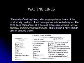
Introduction • Queuing theory is the study of waiting lines • It is one of the oldest and most widely used quantitative analysis techniques • Waiting lines are an everyday occurrence for most people • Queues form in business process as well • The three basic components of a queuing process are arrivals, service facilities, and the actual waiting line • Analytical models of waiting lines can help managers evaluate the cost and effectiveness of service systems
Waiting Line Costs • Most waiting line problems are focused on finding the ideal level of service a firm should provide • In most cases, this service level is something management can control • When an organization does have control, they often try to find the balance between two extremes • A large staff and many service facilities generally results in high levels of service but have high costs
Waiting Line Costs • Having the minimum number of service facilities keeps service cost down but may result in dissatisfied customers • There is generally a trade-off between cost of providing service and cost of waiting time • Service facilities are evaluated on their total expected cost which is the sum of service costs and waiting costs • Organizations typically want to find the service level that minimizes the total expected cost
Cost Service Level Waiting Line Costs • Queuing costs and service level Total Expected Cost Cost of Providing Service Cost of Waiting Time * Optimal Service Level Figure 14.1
Three Rivers Shipping Company Example • Three Rivers Shipping operates a docking facility on the Ohio River • An average of 5 ships arrive to unload their cargos each shift • Idle ships are expensive • More staff can be hired to unload the ships, but that is expensive as well • Three Rivers Shipping Company wants to determine the optimal number of teams of stevedores to employ each shift to obtain the minimum total expected cost
Three Rivers Shipping Company Example • Three Rivers Shipping waiting line cost analysis Optimal cost Table 14.1
Characteristics of a Queuing System • There are three parts to a queuing system • The arrivals or inputs to the system (sometimes referred to as the calling population) • The queue or waiting line itself • The service facility • These components have their own characteristics that must be examined before mathematical models can be developed
Characteristics of a Queuing System • Arrival Characteristics have three major characteristics, size, pattern, and behavior • Size of the calling population • Can be either unlimited (essentially infinite) or limited (finite) • Pattern of arrivals • Can arrive according to a known pattern or can arrive randomly • Random arrivals generally follow a Poisson distribution
where P(X) = probability of X arrivals X = number of arrivals per unit of time = average arrival rate e = 2.7183 Characteristics of a Queuing System • The Poisson distribution is
Characteristics of a Queuing System • We can use Appendix C to find the values of e– • If = 2, we can find the values for X = 0, 1, and 2
0.25 – 0.20 – 0.15 – 0.10 – 0.05 – 0.00 – 0.30 – 0.25 – 0.20 – 0.15 – 0.10 – 0.05 – 0.00 – Probability Probability | 0 | 0 | 1 | 1 | 2 | 2 | 3 | 3 | 4 | 4 | 5 | 5 | 6 | 6 | 7 | 7 | 8 | 8 | 9 | 9 X X = 2 Distribution = 4 Distribution Characteristics of a Queuing System • Two examples of the Poisson distribution for arrival rates Figure 14.2
Characteristics of a Queuing System • Behavior of arrivals • Most queuing models assume customers are patient and will wait in the queue until they are served and do not switch lines • Balking refers to customers who refuse to join the queue • Reneging customers enter the queue but become impatient and leave without receiving their service • That these behaviors exist is a strong argument for the use of queuing theory to managing waiting lines
Characteristics of a Queuing System • Waiting Line Characteristics • Waiting lines can be either limited or unlimited • Queue discipline refers to the rule by which customers in the line receive service • The most common rule is first-in, first-out (FIFO) • Other rules are possible and may be based on other important characteristics • Other rules can be applied to select which customers enter which queue, but may apply FIFO once they are in the queue
Characteristics of a Queuing System • Service Facility Characteristics • Basic queuing system configurations • Service systems are classified in terms of the number of channels, or servers, and the number of phases, or service stops • A single-channel system with one server is quite common • Multichannelsystems exist when multiple servers are fed by one common waiting line • In a single-phase system the customer receives service form just one server • If a customer has to go through more than one server, it is a multiphase system
Queue Departures after Service Service Facility Arrivals Single-Channel, Single-Phase System Queue Type 1 Service Facility Type 2 Service Facility Departures after Service Arrivals Single-Channel, Multiphase System Characteristics of a Queuing System • Four basic queuing system configurations Figure 14.3 (a)
Service Facility1 Departures Queue Service Facility2 after Arrivals Service Facility3 Service Multichannel, Single-Phase System Characteristics of a Queuing System • Four basic queuing system configurations Figure 14.3 (b)
Type 1 Service Facility1 Queue Departures after Service Type 1 Service Facility2 Arrivals Type 2 Service Facility1 Multichannel, Multiphase System Type 2 Service Facility2 Characteristics of a Queuing System • Four basic queuing system configurations Figure 14.3 (c)
Characteristics of a Queuing System • Service time distribution • Service patterns can be either constant or random • Constant service times are often machine controlled • More often, service times are randomly distributed according to a negative exponential probability distribution • Models are based on the assumption of particular probability distributions • Analysts should take to ensure observations fit the assumed distributions when applying these models
– – – – – – – – f (x) | 0 | 30 | 60 | 90 | 120 | 150 | 180 Service Time (Minutes) Characteristics of a Queuing System • Two examples of exponential distribution for service times f (x) =e–xfor x≥ 0 and > 0 = Average Number Served per Minute Average Service Time of 20 Minutes Average Service Time of 1 Hour Figure 14.4
Arrival distribution Service time distribution Number of service channels open Identifying Models Using Kendall Notation • D. G. Kendall developed a notation for queuing models that specifies the pattern of arrival, the service time distribution, and the number of channels • It is of the form • Specific letters are used to represent probability distributions M = Poisson distribution for number of occurrences D = constant (deterministic) rate G = general distribution with known mean and variance
Identifying Models Using Kendall Notation • So a single channel model with Poisson arrivals and exponential service times would be represented by M/M/1 • If a second channel is added we would have M/M/2 • A three channel system with Poisson arrivals and constant service time would be M/D/3 • A four channel system with Poisson arrivals and normally distributed service times would be M/G/4
Single-Channel Model, Poisson Arrivals, Exponential Service Times (M/M/1) • Assumptions of the model • Arrivals are served on a FIFO basis • No balking or reneging • Arrivals are independent of each other but rate is constant over time • Arrivals follow a Poisson distribution • Service times are variable and independent but the average is known • Service times follow a negative exponential distribution • Average service rate is greater than the average arrival rate
Single-Channel Model, Poisson Arrivals, Exponential Service Times (M/M/1) • When these assumptions are met, we can develop a series of equations that define the queue’s operating characteristics • Queuing Equations • We let = mean number of arrivals per time period = mean number of people or items served per time period • The arrival rate and the service rate must be for the same time period
Single-Channel Model, Poisson Arrivals, Exponential Service Times (M/M/1) • The average number of customers or units in the system, L • The average time a customer spends in the system, W • The average number of customers in the queue, Lq
Single-Channel Model, Poisson Arrivals, Exponential Service Times (M/M/1) • The average time a customer spends waiting in the queue, Wq • The utilization factor for the system, , the probability the service facility is being used
Single-Channel Model, Poisson Arrivals, Exponential Service Times (M/M/1) • The percent idle time, P0, the probability no one is in the system • The probability that the number of customers in the system is greater than k, Pn>k
2 cars in the system on the average 1 hour that an average car spends in the system Arnold’s Muffler Shop Case • Arnold’s mechanic can install mufflers at a rate of 3 per hour • Customers arrive at a rate of 2 per hour = 2 cars arriving per hour = 3 cars serviced per hour
1.33 cars waiting in line on the average 40 minutes average waiting time per car percentage of time mechanic is busy probability that there are 0 cars in the system Arnold’s Muffler Shop Case
Arnold’s Muffler Shop Case • Probability of more than k cars in the system
Arnold’s Muffler Shop Case • Input data and formulas using Excel QM Program 14.1A
Arnold’s Muffler Shop Case • Output from Excel QM analysis Program 14.1B
Total service cost Total service cost (Number of channels) x (Cost per channel) = mCs = where m = number of channels Cs = service cost of each channel Arnold’s Muffler Shop Case • Introducing costs into the model • Arnold wants to do an economic analysis of the queuing system and determine the waiting cost and service cost • The total service cost is
Total waiting cost (Total time spent waiting by all arrivals) x (Cost of waiting) = (Number of arrivals) x (Average wait per arrival)Cw = Total waiting cost Total waiting cost = (W)Cw = (Wq)Cw Arnold’s Muffler Shop Case • Waiting cost when the cost is based on time in the system • If waiting time cost is based on time in the queue
Arnold’s Muffler Shop Case • So the total cost of the queuing system when based on time in the system is Total cost = Total service cost + Total waiting cost Total cost = mCs + WCw • And when based on time in the queue Total cost = mCs + WqCw
Total daily waiting cost = (8 hours per day)WqCw = (8)(2)(2/3)($10) = $106.67 • Arnold has identified the mechanics wage $7 per hour as the service cost Total daily service cost = (8 hours per day)mCs = (8)(1)($7) = $56 • So the total cost of the system is Total daily cost of the queuing system = $106.67 + $56 = $162.67 Arnold’s Muffler Shop Case • Arnold estimates the cost of customer waiting time in line is $10 per hour
1 car in the system on the average 1/2 hour that an average car spends in the system Arnold’s Muffler Shop Case • Arnold is thinking about hiring a different mechanic who can install mufflers at a faster rate • The new operating characteristics would be = 2 cars arriving per hour = 4 cars serviced per hour
1/2 cars waiting in line on the average 15 minutes average waiting time per car percentage of time mechanic is busy probability that there are 0 cars in the system Arnold’s Muffler Shop Case
Arnold’s Muffler Shop Case • Probability of more than k cars in the system
Total daily waiting cost = (8 hours per day)WqCw = (8)(2)(1/4)($10) = $40.00 • The new mechanic is more expensive at $9 per hour Total daily service cost = (8 hours per day)mCs = (8)(1)($9) = $72 • So the total cost of the system is Total daily cost of the queuing system = $40 + $72 = $112 Arnold’s Muffler Shop Case • The customer waiting cost is the same $10 per hour
Arnold’s Muffler Shop Case • The total time spent waiting for the 16 customers per day was formerly (16 cars per day) x (2/3 hour per car) = 10.67 hours • It is now is now (16 cars per day) x (1/4 hour per car) = 4 hours • The total system costs are less with the new mechanic resulting in a $50 per day savings $162 – $112 = $50
Enhancing the Queuing Environment • Reducing waiting time is not the only way to reduce waiting cost • Reducing waiting cost (Cw) will also reduce total waiting cost • This might be less expensive to achieve than reducing either W or Wq
Multichannel Model, Poisson Arrivals, Exponential Service Times (M/M/m) • Assumptions of the model • Arrivals are served on a FIFO basis • No balking or reneging • Arrivals are independent of each other but rate is constant over time • Arrivals follow a Poisson distribution • Service times are variable and independent but the average is known • Service times follow a negative exponential distribution • Average service rate is greater than the average arrival rate
Multichannel Model, Poisson Arrivals, Exponential Service Times (M/M/m) • Equations for the multichannel queuing model • We let m = number of channels open = average arrival rate = average service rate at each channel • The probability that there are zero customers in the system
Multichannel Model, Poisson Arrivals, Exponential Service Times (M/M/m) • The average number of customer in the system • The average time a unit spends in the waiting line or being served, in the system
Multichannel Model, Poisson Arrivals, Exponential Service Times (M/M/m) • The average number of customers or units in line waiting for service • The average number of customers or units in line waiting for service • The average number of customers or units in line waiting for service
probability of 0 cars in the system Arnold’s Muffler Shop Revisited • Arnold wants to investigate opening a second garage bay • He would hire a second worker who works at the same rate as his first worker • The customer arrival rate remains the same