Waiting Lines

1. Waiting Lines Quantitative Module: Part D

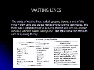
2. Waiting Lines: What and Why? • A waiting line is one or more “customers” or items queued for operation, which can include people waiting for service, materials waiting for further processing, equipment waiting for maintenance, and sales order waiting for delivery. • Forms because of temporary imbalance between the demand for service and the capacity of the system to provide service.

3. Why is there waiting? Occurs naturally because of two reasons: • Customers arrive randomly, and not at evenly placed times nor at predetermined times. • Service requirements of customers are variable, and not uniform. (Teller counter of a Bank). Both Arrival & Service times exhibit a high degree of variability. Leads to: Over-loaded Systems Under-loaded Systems Waiting Lines formation No Waiting Line

4. Goal of Waiting-Line Analysis • Minimize Total Cost. • Cost of customer waiting for service. • Capacity cost to provide service. Total cost Customer waiting cost Capacity cost = + Total cost Cost of service capacity Cost Cost of customers waiting Service capacity Optimum

5. System Characteristics • Population Source. • Number of Servers. • Arrival Pattern. • Queue Discipline. • Service Pattern.

6. Population Source • Finite-source: • Limited size of the customer pool. • Entry / Exit by a member of this population pool will affect the probability of a customer requiring service. • E.g.: A machine in a company. The potential number of machines that might need repair at any one time cannot exceed the number of machines. • Infinite-source: • Sufficiently large customer pool. • Any change in population size caused by subtractions or additions to the population does not affect the system prob. • E.g.: 100 machines being maintained by one repairperson. A department store that has 10,000 customers.

7. Number of Servers • System-Capacity is a function of: • Server Capacity. • Number of Servers in the system. Single Channel, Single Phase Single Channel, Multiple Phase Multiple Channel, Single Phase Multiple Channel, Multiple Phase

8. Arrival Patterns Arrival rate: • The average number of customers or units per time period. • Constant: exactly the same time period between successive arrivals. E.g. machine controlled production process. • Random (Variable): When arrivals are independent of each other and their occurrence cannot be predicted. • This variability can be described by theoretical distributions. • Most common for arrival rate is Poisson Distribution.

9. Poisson Distribution Probability 0 1 2 3 4 5 6 7 8 9 0 1 2 3 4 5 6 7 8 9 10 11 Distribution for λ = 2 Distribution for λ = 4

10. Service Pattern Service Time: • The average time to process one customer. • Constant: exactly the same time to process each customer (order). E.g. automated car wash. • Random (Variable): When exact service times cannot be predicted. Most require short processing times, but some could require relatively long service times. • This variability can be described by theoretical distributions. • Most common for arrival rate is Exponential Distribution.

11. Exponential Distribution Average service rate (µ ) = 3 customers /hr. Probability that service time ≥ t Average service rate (µ ) = 1 customer /hr. Time t in hours

12. Measures of System Performance • Average time that each customer or object spends in the queue. • Average queue length. • Average time that each customer spends in the system (waiting time plus service time). • Average number of customers in the system. • Probability that the service facility will be idle. • Utilization factor for the system. • Probability of a specific number of customers in the system.

13. Waiting Line Models • Infinite-Source: • Single Channel, Exponential Service Time. Model 1. • Single Channel, Constant Service Time. Model 2. • Multiple Channel, Exponential Service Time. Model 3. • Multiple Channel with priority service. Exponential service time. Model 4. (NOT COVERED IN THIS COURSE) • Finite-Source:

14. Infinite-Source Symbols

15. Basic Relationships

16. Model 1: S.C. & E.S.T. Is the Simplest model, which involves: One server (single crew). Arrival rates are Poisson. First-come, first-served. Service times are Exponential.

17. Example A phone company is planning to open a satellite store in a new shopping mall, staffed by one sales agent. It is estimated that requests for phones, accessories, and information will average 15 per hour, and requests will have a Poisson distribution. Service times is assumed to be Exponentially distributed. Previous experience with similar satellite operations suggests that mean service time should average about three minutes per request. Determine each of the following: • System utilization. • Percentage of time the sales agent will be idle. • The expected number of customers waiting to be served. • The average time customers will spend in the system. • The probability of zero customers in the system and the probability of four customers in the system.

18. Model 2: S.C. & C.S.T. • Exactly similar to Model 1, except that service time is not variable. • Constant Service Time. • Cuts the average number of customers waiting in line by half. • All the formulas are the same as in Model 1, except:

19. Example Wanda’s Car Wash & Dry is an automatic, five-minute operation with a single bay. On a typical Saturday morning, cars arrive at a mean rate of eight per hour, with arrivals tending to follow a Poisson distribution. Find: • The average number of cars in line. • The average time cars spend in line and service.

20. Model 3: M.C. & E.S.T. • 2 or more servers working independently to provide service. • Poisson arrival rate and Exponential service time. • All servers work at the same average rate. • Customers form a single waiting line (FCFS).

21. Can also use Table 19-4 on page: 787-788.

22. Example Alpha Taxi and Hauling Company has seven cabs stationed at the airport. The company has determined that during the late-evening hours on weeknights, customers request cabs at a rate that follows the Poisson distribution with a mean of 6.6 per hour. Service time is exponential with a mean of 50 minutes per customer. Assume that there is one customer per cab and that each taxi returns to the airport after dropping off the passenger. Find: • Average number of customers waiting in line. • Probability of zero customers in the system. • Probability of 3 customers and 10 customers in the system. • Average waiting time for an arrival not immediately served. • Probability that an arrival will have to wait for service. • System utilization.

23. Example Trucks arrive at a warehouse at an average rate of 15 per hour during business hours. Crews can unload the trucks at an average rate of five per hour. (Both distributions are Poisson). The high unloading rate is due to cargo being put into containers. Recent changes in wage rates have caused the warehouse manager to re-examine the question of how many crews to use. The new rates are: crew and dock cost $100 per hour; truck and driver cost $120 per hour.

24. Examples • Repair calls for Xerox copiers in a small city are handled by one repairman. Repair time, including travel time, is exponentially distributed, with a mean of two hours per call. Requests for copier come in at a mean rate of three per eight-hour day (assume Poisson). Assume infinite source. Determine: • The average number of copiers awaiting repairs. • System utilization. • The amount of time during an eight-hour day that the repairman is not out on a call. • The probability of two or more copiers in the system (waiting or being repaired).

25. Examples • A vending machine dispenses hot chocolate or coffee. Serving time is 30 seconds per cup and is constant. Customers arrive at a mean rate of 80 per hour, and this rate is Poisson-distributed. Assume that each customer buys only one cup. Determine: • The average number of customers waiting in line. • The average time customers spend in the system. • The average number of customers in the system.

26. Examples • Many of a bank’s customers use its automated teller machine (ATM) to transact business. During the early evening hours in the summer months, customers arrive at the ATM at the rate of one every other minute. This can be modeled using a Poisson distribution. Each customer spends an average of 90 seconds completing his or her transactions. Transaction time is exponentially distributed. Determine: • The average time customers spend at the machine, including waiting in line and completing transactions. • The probability that a customer will not have to wait upon arrival at the ATM. • Utilization of the ATM.

27. Examples • A small town with one hospital has two ambulances to supply ambulance service. Requests for ambulances during weekdays mornings average 0.8 per hour and tend to be Poisson-distributed. Travel and loading/unloading time averages one hour per call and follows an exponential distribution. Find: • System utilization. • The average number of customers waiting. • The average time customers wait for an ambulance. • The probability that both ambulances will be busy when a call comes in.

28. Examples • The manager of a regional warehouse must decide on the number of loading docks to request for a new facility in order to minimize the sum of dock-crew and driver-truck costs. The manager has learned that each driver-truck combination represents a cost of $300 per day and that each dock plus loading crew represents a cost of $1,100 per day. • How many docks should be requested if trucks arrive at the rate of four per day, each dock can handle five trucks per day, and both rates are Poisson? • An employee has proposed adding new equipment that would speed up the loading rate to 5.71 trucks per day. The equipment would cost $100 per day for each dock. Should the manager invest in the new equipment?

29. Additional Examples • Trucks are required to pass through a weighing station so that they can be checked for weight violations. Trucks arrive at the station at the rate of 40 an hour between 7 p.m. and 9 p.m. according to Poisson distribution. Currently two inspectors are on duty during those hours, each of whom can inspect 25 trucks an hour. Assume service times to be exponentially distributed. • How many trucks would you expect to see at the weighing station, including those being inspected? • If a truck were just arriving at the station, about how many minutes could the driver expect to wait? • How many minutes, on average, would a truck that is not immediately inspected have to wait? • What is the probability that both inspectors would be busy at the same time? • What condition would exist if there were only one inspector?

30. The parts department of a large automobile dealership has a counter used exclusively for mechanics’ requests for parts. The time between requests can be modeled by an Exponential distribution that has a mean of five minutes. A clerk can handle requests at a rate of 15 per hour, and this can be modeled by a Poisson distribution. Suppose there are two clerks at the counter. • On average, how many mechanics would be at the counter, including those being served? • If a mechanic has to wait, how long would the average wait be? • What is the probability that a mechanic would have to wait for service? • What percentage of time is a clerk idle? • If clerks represent a cost of $20 per hour and mechanics a cost of $30 per hour, what number of clerks would be optimal in terms of minimizing total cost?

31. Trucks arrive at the loading dock of a wholesale grocer at the rate of 1.2 per hour in the mornings. A single crew consisting of two workers can load a truck in about 30 minutes. Crew members receiver $10 per hour in wages and fringe benefits, and trucks and drivers reflect an hourly cost of $60. The manager is thinking of adding another member to the crew. The service rate would then be 2.4 trucks per hour. Assume rates are Poisson. • Would the third crew member be economical? • Would a fourth member be justifiable if the resulting service capacity were 2.6 trucks per hour?