Waiting Lines
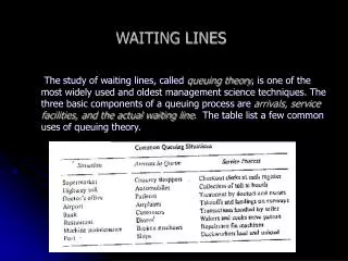
Waiting Lines. Why do Queues Exist?. Uncertainty: Time between arrivals of customers Time to serve a customer. Servers. Customer. A queue is an inventory of demand. Waiting Line (Queueing) Models. Queuing theory : Mathematical approach to the analysis of waiting lines.


Waiting Lines
E N D
Presentation Transcript
Why do Queues Exist? Uncertainty: • Time between arrivals of customers • Time to serve a customer Servers Customer A queue is an inventory of demand.
Waiting Line (Queueing) Models • Queuing theory: Mathematical approach to the analysis of waiting lines. • What are queueing models? • Why should we study queueing models?
Waiting Line (Queueing) Models • What are the key performance measures of queueing sytsems? • How to analyze these performance measures? • What are the applications of queueing models?
What are Queueing Models? Queueing Models are characterized by (1) arriving customers, (2) service facility and servers, (3) the way customers are served. servers Customers Wait here
Basic Elements of Queueing Systems Server Operation Customer Arrival System Configuration Queueing Models System Performance (avg. # of customers waiting, avg. waiting time in line)
Processing order Arrivals Waiting line Service Exit System Basic Elements of a Queuing System
Examples of Waiting Lines • Banks, Toll booths, Emergency Rooms, Amusement Parks, Immigration Department, … etc. • Computer Systems, Hot Lines, Telecommunication Systems, Production Systems, ...etc.
Why should we study queueing models? • To analyze the efficiency of a service facility • waiting time, No. of customers waiting • To improve the design of a service system • reduce waiting time, improve service quality • Improve the quality of a service system • Good service can improve reputation, increase market share
How do we measure a queueing system? (System Performance) • Average number of customers waiting • Average time customers wait • System utilization: % of capacity utilized • Probability that an arrival will have to wait
System Configuration • Single server • Mutiple servers • Single Line • Multiple Lines
System Configuration • Queue Discipline • FIFO (FCFS): first-in-first-out (first-come-first-served) • LIFO (LCFS): last-in-first-out (last-come-first-served) • Priority
Queuing Models • Single channel, general service time (M/G/1) • Single channel, exponential service time (M/M/1) • Single channel, constant service time (M/D/1) • Multiple channel, exponential service time (M/M/c) • Multiple priority service
Notations • Notations used are slightly different from that of the text book. • M/M/k No. of servers Service time distribution, M stands for exponential, G for general Customer arrival pattern, M stands for customers arriving the system following a Poisson pattern, or equivalently, the inter-arrival time between consecutive customers has an exponential distribution.
Poisson Distribution Example: Horse Kick in the Prussian Army In 1898, Ladislaus von Bortkiewicz performed one of the most unusual “field exercises.” Bortkiewicz compiled the Prussian army records of the number of men killed by a horse kick in each of 10 cavalry units or corps in each of 20 successive years (1875-1894). He took the number of men killed in each corps in each year as a single observation. With 10 corps and 20 years this gave him a total of 200 observations. There were a total of 122 deaths or an average of 122/200 =0.61 deaths per corps per year. He then compared the actual frequency of deaths in each corps in each year to a theoretical Poisson distribution with mean = 0.61. The results are shown in the table on next page. For example, there were 22 instances of two deaths in a corps in a single year. The actual observations and the Poisson predictions are remarkable close.
Notations (continued) : Customer arrival rate (No. of arrivals per unit time) : Service rate; ms = 1/ : mean service time (per customer) L: Average number of customers in the system (waiting + being serviced) Lq: Average number of customers in the queue (waiting for service) W: Average time of a customer spent in the system (throughput time) Wq: Average time of a customer spent in the queue (waiting or queue time) : System utilization rate; = / for single server and = /(c) for multiple servers. : Standard deviation of service time
How to find performance measures? • Performance measures are refered to the long-run or steady-state performance measures of the system. They can be found by the following approaches: • Laws • Queueing Formulas • Simulation
Queueing “Laws” • Pipeline Principle • Average output equals to average input in a stable system: • Throughput rate = • Little’s Law: • L = W • Lq = Wq • Additivity of time: throughput time equals service time plus waiting time: • W = ms + Wq = 1/ + Wq
Queueing “Laws” (continued) • Using Little’s Law and the Law of additivity of time, we can calculate all the performance measures if we can find any one of them. If we multiple the formula of additivity of time by , we get • L = / + Lq Notice that Lq is the number of customers waiting in the system and /gives the average number of customers being served in the system at any point of time.
System Configuration • Single server (Single channel) wait here
M/G/1 system • Utilization rate: = ms= / < 1. • Pollaczek-Khintchine Formula: “Excess” capacity is a necessary condition to maintain the throughput time performance. If the customers arrival rate increases so as to equal to the service rate, the system will explode. The system will never attain steady state if / 1. Stochastic variability in the arrival pattern and customer service requirements causes congestion and delay. More variability is worse.
Example A company is considering three options for order processing: a manual system, two computer systems (CS1 and CS2). Customers arrive according to a Poisson process at the rate of 15 per hour. The relevant data are given in the following table:
Example - solutions Manual system: = 15/60 = 0.25 customer per minute. Remember to use the same time unit! ms = 3 min. System utilization: = / = (0.25)(3.0) = 0.75. Lq = 2( (ms)2 + 2)/{2(1- )} = (0.25)2{3.02 + 9.0) / {2(1 - 0.75)} = 2.25 customers, Wq = Lq/ = 2.25/0.25 = 9 minutes, W = Wq + ms = 9 + 3 = 12 minutes, L = W = 0.25 12 = 3 customers.
Example - solutions CS1: System utilization: = (0.25)(3.0) = 0.75. Lq = (0.25)2{3.02 + 4.5) / {2(1 - 0.75)} = 1.6875 customers, Wq = Lq/ = 1.6875/0.25 = 6.75 minutes, W = Wq + ms = 6.75 + 3 = 9.75 minutes, L = W = 0.25 9.75 = 2.4375 customers.
Example - solutions CS2: System utilization: = (0.25)(3.1) = 0.775. Lq = (0.25)2{3.12 + 1.0) / {2(1 - 0.775)} = 1.4736 customers, Wq = Lq/ = 1.4736/0.25 = 5.8944 minutes, W = Wq + ms = 5.8944 + 3.1 = 8.9944 minutes, L = W = 0.25 8.9944 = 2.2486 customers.
M/M/1 system If < 1, then the steady state performance of the system is given by:
Example - p.818 An airline is planning to open a satellite ticket desk in a new shopping plaza, staffed by one ticket agent. It is estimated that requests for tickets and information will average 15 per hour, and requests will have a Poisson distribution. Service time is assumed to be exponentially distributed. Previous experience with similar satellite operations suggests that mean service time should average about three minutes per request. Determine (a) Percent of time the server will be idle; (b) the expected number of customers waiting to be served; ( c ) the average time customers will spend in the system; (d) the probability of no customer in the system; (e) the probability of more than two customers in the system.
Example - solution = 15 customers per hour; = 20 customers per hour. (a). = 15/20 = 0.75; Percentage of idle time = 1 - = 0.25 = 25% (b). Lq = 2/{( - )} = 15 2 /{20(5)} = 2.25 customers. (c). W = 1/( - ) = 1/5 hour = 12 minutes. (d). p0 = 1 - = 0.25. (e). p1 = p0 = (0.75)(0.25) = 0.1875 ; p2 = 2p0 = (0.75)2(0.25) = 0.1406 ; Prob{more than 2 customers in system} = 1 - p0 - p1 - p2 = 1 - 0.25 - 0.1875 - 0.1406 = 0.4219
System Configuration (multiple server) wait here Independent System wait here Pooling System
M/M/c model • Important: the textbook uses M to denote the number of servers and I use c to denote it. • The performance measures for this model is given in Table 17-3 (p.820) and their values for different values of the system parameters are given in Table 17-4 (pp.820-822).
M/M/c model - Example Two managers, each produces = 4 documents per hour. The company hire two typists, each can type = 5 documents per hour. Assuming each manager generates documents according to a Poisson pattern and the time a typists needed to finish a document follows an exponential distribution. Compare the alternatives of assigning a typists to each manager or “pooling” the typists for the two managers.
M/M/c Example - solutions Case 1: Two independent lines, i.e., each typist is assigned to a manager and will not work for the other manager. In this case, each line is a M/M/1 model. = / = 4/5 = 0.8. (Utilization rate for each system) W = 1/( - ) = 1 hour. Wq = /{ /( - )} = 0.8 hour L = W = 4 customers. Lq = Wq = 4(0.8) = 3.2 customers (documents)
M/M/c Example - solutions (continued) Case 2: Pooling: The typists will type the documents according to the FIFO rule. In this case, = 8, = 5. System utilization: = 8 / (2 5) = 0.8 From Table 17-4 of Chapter 17: Lq = 2.844, Wq = Lq/ = 2.844/8 = 0.356. L = / + Lq = 1.6 + 2.844 = 4.444, W = L/ = 0.5556
Economies of scales in service systems • In the M/M/1 model, if both the arrival rate and the service rate are increased by 100%. Let Wq(new) and Wq(old) denote the new and old performance measures. Then On the average, the waiting time for a customer in the new system is only 50% of that in the old system. What happen to the other measures?
Economies of scales in service systems • In the M/M/2 example we have discussed, a document requires only 0.556 hour to be finished (waiting plus typing), a reduction of over 45% from the independent system. Only 2.8444 (Lq) documents are waiting in the system on the average, while in the independent systems, there are 3.2 + 3.2 = 6.4 documents waiting in the system.
Economies of scales in service systems • In the independent system, the percentage idle time of a typist is 20% ( 1 - ). • In the pooling system, p0 = 0.111 (Table 17-4); we can also evaluate p1 = 0.1776 (from formula). Thus the average idle time for a typist in the pooling system is {2p0 + p1}/2 = 0.1999 = 20%. • The typists are working as hard in both systems.
Economies of scales in service systems • In the independent system, a document spends 0.8 hours waiting on the average before it is typed by a typist, compare with only 0.3556 hour in the pooling system. A reduction of over 54% in the new system. • Notice that the improvement in the new system requires NO EXTRA investment. It just requires you to analyze the different alternatives and perform some management rearrangement (Business Process Reengineering). One of the focal points of Operations Management.
Waiting Time vs Utilization Average number or time waiting in line 100% 0 System Utilization
Queuing Analysis Total cost Customer waiting cost Capacity cost = + Cost Total cost Cost of service capacity Cost of customers waiting Service capacity Optimum
System Characteristics • Population Source • Infinite source: customer arrivals are unrestricted • Finite source: number of potential customers is limited • Number of observers (channels) • Arrival and service patterns • Queue discipline (order of service)
System Performance • Average number of customers waiting • Average time customers wait • System utilization • Implied cost • Probability that an arrival will have to wait Measured by:
Processing order Arrivals Waiting line Service Exit System Priority Model 1 3 2 1 1 Arrivals are assigned a priority as they arrive
Finite-Source Queueing The models we have considered above assumed that the population (of customers) is infinite (What is the characteristic?). There is another class of useful queueing models: The finite source (or population) queueing models. This class of model is very useful in the maintenance and repairing management of machines and expensive equipment.
Managing service systems • General Principles: • Reduce variability • Increase flexibility • Better planning and scheduling
Managing service systems • Smooth Arrivals • Customer appointments/reservations • Schedule reliable vendor/suppliers • Smooth demand by pricing, advertising, promotion and subcontracting • Acquire more information about customers.
Managing service systems • Increase capacity or improve technology • Pooling: capacity sharing/flexible training • Reduce mean service time • better training • improve procedures • new technology/automation • specialization
Managing service systems • Reduce variability in processing time • limited variability • uniform processing • specialization: division of labor/exploit customer heterogeneity.
Managing service systems • Reduce the impact/cost of waiting • Scheduling policies: priority rules • reduce the impact of waiting • the more valuable the service, the longer will people wait • Preprocess waits feel longer than in-process waits. • Anxiety makes waits seem longer. • Unfair waits are longer than equitable waits. • Uncertain waits are longer than known waits. • Unexplained waits are longer than explained waits • Unoccupied waits are longer than occupied waits. • Solo waits feel longer than group waits.