Download
1 / 49
490 likes | 881 Vues
Estimating regional C fluxes by exploiting observed correlations between CO and CO 2. Paul Palmer Division of Engineering and Applied Sciences Harvard University. http://www.people.fas.harvard.edu/~ppalmer. + ballpark flux estimates for fast exchange processes (10 9 tonnes C). 61. 60. 1.6.

E N D
Estimating regional C fluxes by exploiting observed correlations between CO and CO2 Paul Palmer Division of Engineering and Applied Sciences Harvard University http://www.people.fas.harvard.edu/~ppalmer
+ ballpark flux estimates for fast exchange processes (109 tonnes C) 61 60 1.6 5.5 IPCC
? China GDP (Billion 1995 yuan constant) Year China Energy Databook v6, 2004 IPCC Chinese Government Statistics Shown Downward Trend in Chinese CO2 Emissions (Streets et al., Science, 294, 1835-1837, 2001)
Bottom-up Emission Inventories are Very Uncertain Emission Factor (TgC / Tg fuel) Emissions (Tg C yr-1) E = AF Coal-burning cook stoves in Xian, China Activity Rate (Tg fuel yr-1) (amount of fuel burned)
Remote data have limitations in estimating regional C budgets RH + OH … CO CO2 Direct & indirect emissions Many 100s km 10s km CMDL site 1000s km Increasing model transport error
Aircraft data can improve level of disaggregation of continental emissions Feb – April 2001 NASA TRACE-P Main transport processes: • DEEP CONVECTION • OROGRAPHIC LIFTING • FRONTAL LIFTING warm air cold air cold front
Offshore China Over Japan Slope (> 840 mb) = 22 R2 = 0.45 Slope (> 840 mb) = 51 R2 = 0.76 ATMOSPHERIC CO2:CO CORRELATIONS PROVIDE UNIQUE INFORMATION ON SOURCE REGION AND TYPE A priori bottom-up CO2 CO2 CO CO Top-down - CO2:CO emission ratios vary with combustion efficiency - Range in regional emission ratios reflect mix of sources and variation in fossil fuel combustion ratio Suntharalingam et al, 2004
Modeling Overview Forward model (GEOS-CHEM) Inverse model ^ x = xa + (KTSy-1K + Sa-1)-1 KTSy-1(y – Kxa) y = Kxa + State vector (Emissions x) Observation vector y x = Fluxes of CO and CO2 from Asia (Tg C/yr) y = TRACE-P CO and CO2 concentration data
Consistent CO and CO2 Emissions Inventories Biomass burning: Variability from observed daily firecount data (AVHRR) Heald et al, 2003 Anthropogenic emissions for 2001: domestic ff, biofuel, transport, industrial ff Streets et al, 2003
Seasonal Cycle of Chinese CO and CO2 Emissions during TRACE-P TERRESTIAL BIOSPHERE: CASA (Randerson, et al, 1997) OCEAN BIOSPHERE: Takahashi et al, 1999 TOTAL TOTAL CO BIOFUEL FOSSIL Gt C yr-1 Fraction of annual emissions BIOBURN BIOSPHERE Annual Mean TRACE-P Streets et al, 2003
Estimating the Jacobian Global 3D CTM 2x2.5 deg resolution Boreal Asia (BA) China (CH) Japan (JP) Rest of World (ROW) Korea (KR) x = emissions from individual countries and individual processes (BB, BF, FF) Southeast Asia (SEA) [OH] from full-chemistry model (CH3CCl3 = 6.3 years)
TRACE-P Observations Remove CO2 bias using 10th percentile of [CO2]: 4-4.5 ppm GEOS-CHEM 4-6 km 2-4 km CO [ppb] CO2 [ppm] 0-2 km Latitude [deg]
^ x = xa + (KTSy-1K + Sa-1)-1 KTSy-1(y – Kxa) S = (KTSy-1K + Sa-1)-1 Xs = retrieved state vector (the CO sources) Xa= a priori estimate of the CO sources Sa = error covariance of the a priori K = forward model operator Sy = error covariance of observations = instrument error + model error + representativeness error Gain matrix ^ Linear Inverse Model
GEOS-CHEM All latitudes RRE Mean bias TRACE-P GEOS-CHEM 2x2.5 cell Altitude [km] (measured-model) /measured Error specification for CO and CO2 SaAnthropogenic (c/o Streets): China (78%), Japan (17%), Southeast Asia (100%), Korea (42%) – uniform 25%Biomass burning: 50% 30%Chemistry (~CH4): 25% Biosphere: 75% SyMeasurement accuracyRepresentation Model error (most important) RRE = total observation error (y*RRE)2 ~38ppb (CO) ~1.87ppm (CO2) CO
NUMBER OF EIGENVALUES OF PREWHITENED JACOBIAN 1 = DOF ~ -1/2 1/2 K =S KS a Rodgers, 2000 CO: CH ANTH*, KRJP&, SEA, CH BB, BA BB@, ROW CO2: CH ANTH*, KRJP&, CH BB$, BA BB@, BS, ROW (inc SEA$) *Collocated sources; &coarse resolution forces merging; $observed gradients too weak to resolve source; @not well resolved
Independent Inversion of CO and CO2 emissions A priori A posteriori Anthropogenic CO2 CO emissions [Tg yr-1] Biospheric CO2 K ~ CO2 emissions [Tg March 2001] 1 Results consistent with [CO2]:[CO] analysis
Japan China Slope (> 840 mb) = 22 R2 = 0.45 Slope (> 840 mb) = 51 R2 = 0.76 Offshore China Over Japan 50% CO increase from inverse model not enough Reconciliation with observations: decrease a CO2 source withhigh CO2:CO CO2/CO Observed CO2:CO correlations are consistent with Chinese biospheric emissions of CO2 40% too high • Problem: Modeled Chinese CO2:CO slopes are 50% too large biosphere Suntharalingam et al, 2004
^ C A posteriori correlation matrix illustrates the ambiguity between anthropogenic and biospheric CO2 emissions Chinese anthropogenic CO2 Chinese biospheric CO2 CO2 state vector
N N Modeling correlations between CO and CO2 ECO = (A + AA) (FCO + COFCO) ECO2 = (A + AA) (FCO2 + CO2FCO2) Carbon Conservation (CO+CO2 ~ 0.9-1.0) Perturbed F 0.9 1 Unperturbed F
A >> F A << F Interpretation of correlations F F A CO2 Emissions CO2 Emissions A CO Emissions CO Emissions r > 0 r < 1
VALUES OF UNCERTAINTY FROM STREETS’ INCONSISTENT WITH DATA ANALYSIS AND LEAD TO SMALL CO2:CO CORRELATIONS E = AF A: CO 5-25%; CO2 5-20% F: CO 50 - 200%; CO2 5-10% Correlations: China ~0 Korea/Japan -0.2 Southeast Asia ~0 Correlations within sectors > lumped sectors
Alternative Correlations Tested… Streets’ Min(A 25%) Min(A 50%) CO2:CO Correlation Korea + Japan Southeast Asia Chinese anthropogenic Also r = 0.5,…,1.0
A correlation of > 0.7 is needed to start decoupling biospheric and anthropogenic CO2 Anthropogenic CO2 Anthropogenic CO A posteriori Uncertainty [unit] Biospheric CO2 Lowest correlations correspond to those calculated using Monte Carlo method
Future satellite missions The “A Train” 1:38 PM 1:30 PM 1:15 PM Aura Cloudsat OCO CALIPSO Aqua PARASOL OCO - CO2 column OMI - Cloud heights OMI & HIRLDS – Aerosols MLS& TES- H2O & temp profiles MLS & HIRDLS – Cirrus clouds CALPSO- Aerosol and cloud heights Cloudsat - cloud droplets PARASOL - aerosol and cloud polarization OCO - CO2 MODIS/ CERES IR Properties of Clouds AIRS Temperature and H2O Sounding • Due for launch in 2004 • IR, high res. Fourier spectrometer (3.3 - 15.4 mm) • Has 2 viewing modes: nadir and limb • Spatial resolution of nadir view = 8x5 km2 C/o M. Schoeberl
New Concept: Testing science objectives of satellite instruments before launch Orbiting Carbon Observatory (OCO) Tropospheric Emission Spectrometer (TES) • Launch date in 2007. • Will provide column CO2 measurements • 3 spectrometers that measure CO2 at 1.61m and 2.05m and O2 at 0.76m • Field of view of spectrometers is 1x1.5 km2 • Sun-synchronous orbit with 16-day repeat cycle and 1:15 pm equator crossing time • Launched in July 2004 • An IR, high resolution Fourier spectrometer • Measures spectral range 3.3 - 15.4m • Limb and nadir view (footprint is 8x5 km2) • Sun-synchronous orbit with 16-day repeat cycle Will measurements of CO and CO2 from TES and OCO provide accurate constraints on carbon fluxes from different regions in Asia? Jones et al, 2004
Simulation: Constraining Asian Carbon Fluxes from Space Generate pseudo-data from the satellites for March 1-31, 2001 CO (825 mb) along TES orbit (1 day) CO2 column along OCO orbit (1 day) ppm ppb Inverse model with realistic instrument and model errors, and which accounts for data loss due to cloud cover and the vertical sensitivity of the instruments Jones et al, 2004
BorealAsia BB BorealAsia BB BorealAsia BB BorealAsia BB BorealAsia BB BorealAsia BB BorealAsia BB BorealAsia BB BorealAsia BB IndiaFuel IndiaFuel IndiaFuel IndiaFuel IndiaFuel IndiaFuel IndiaFuel IndiaFuel IndiaFuel JP/KRFuel JP/KRFuel JP/KRFuel JP/KRFuel JP/KRFuel JP/KRFuel JP/KRFuel JP/KRFuel JP/KRFuel SE AsiaFuel SE AsiaFuel SE AsiaFuel SE AsiaFuel SE AsiaFuel SE AsiaFuel SE AsiaFuel SE AsiaFuel SE AsiaFuel India BB India BB India BB India BB India BB India BB India BB India BB India BB ChinaBB ChinaBB ChinaBB ChinaBB ChinaBB ChinaBB ChinaBB ChinaBB ChinaBB SE Asia BB SE Asia BB SE Asia BB SE Asia BB SE Asia BB SE Asia BB SE Asia BB SE Asia BB SE Asia BB ChinaFuel ChinaFuel ChinaFuel ChinaFuel ChinaFuel ChinaFuel ChinaFuel ChinaFuel ChinaFuel Japan Korea Japan Korea Japan Korea Japan Korea Japan Korea Japan Korea Japan Korea SE Asia SE Asia SE Asia SE Asia SE Asia SE Asia SE Asia Rest of world Rest of world Rest of world Rest of world Rest of world Rest of world Rest of world India India India India India India India China China China China China China China Boreal Asia Boreal Asia Boreal Asia Boreal Asia Boreal Asia Boreal Asia Boreal Asia Significant reduction in uncertainty in estimates of the dominant Asian biospheric fluxes (China and Boreal Asia) A Posteriori Error Estimates [%] CO Sources A priori A priori A priori A priori A priori A priori A priori A posteriori A posteriori A posteriori A posteriori A posteriori A posteriori A posteriori CO2 Sources Biospheric CO2 Chinese biospheric fluxes weakly coupled to anthropogenic emissions Jones et al, 2004
Closing Remarks • Estimated Chinese anthropogenicCO(CO2) sources are currently too low (high). • Chinese biospheric CO2 fluxes are estimated too high but they are coupled to anthropogenic CO2. Correlations between CO2 and CO can decouple these signals. • Emission correlations summed over sectors are too weak – need r > 0.7, impossible with current inverse model configuration. • Work in progress – much still to explore.
Increased Domestic Coal Fractional Increase in Residential Coal Sector A Fractional Increase in Chinese Anthropogenic CO2 Emissions Increased Biofuel Fractional Increase in Biofuel Sector A CO2:CO analysis shows that A and F responsible for E Adjusting only E unrealistic values: 15/30% for biofuel and domestic coal Suntharalingam et al, 2004
Domestic coal Biofuel Transport r=-0.13 n = 16893 r=-0.0019 n = 11387 r=-0.43 n = 4754 CO2 Emissions Industrial Coal Lumped sectors r=-0.12 n = 13954 r=-0.03 n = 4754 CO Emissions Correlations within sectors > lumped sectors e.g., China Low or negative correlations reflect relatively large uncertainties in emission factors
Improvements to Inverse Model xs = xa + (KTSy-1K + Sa-1)-1 KTSy-1(y – Kxa) SS = (KTSy-1K + Sa-1)-1 Xs = retrieved state vector (the CO sources) Xa= a priori estimate of the CO sources Sa = error covariance of the a priori K = forward model operator Sy = error covariance of observations = instrument error + model error + representativeness error Gain matrix • Choice of x… • Aggregate anthropogenic emissions (colocated sources) • Aggregate Korea/Japan (coarse model grid resolution)
IPCC Chinese Government Statistics Shown Downward Trend in Chinese CO2 Emissions (Streets et al., Science, 294, 1835-1837, 2001)
CO inverse modeling • Product of incomplete combustion; main sink is OH • Lifetime ~1-3 months • Relative abundance of observations CMDL network for CO and CO2 • Big discrepancy between Asian emission inventories and observations TRACE-P (Transport And Chemical Evolution over the Pacific) data can improve level of disaggregation of continental emissions
Seasonal cycles of CO2 sources Biospheric emissions are 65% of Chinese total, according to bottom-up inventories Gt C yr-1 TRACE-P
Fuel consumption(Streets) Biomass burning AVHRR (Heald/Logan) Global 3D CTM 2x2.5 deg resolution China Japan Korea Southeast Asia Rest of World [OH] from full-chemistry model (CH3CCl3 = 6.3 years) x = emissions from individual countries and individual processes (BB, BF, FF)
Removal of CO2 model bias Modeled Observed
ATMOSPHERIC CO2:CO CORRELATIONS PROVIDE UNIQUE INFORMATION ON SOURCE REGION AND TYPE Regional CO2/CO Emissions Ratios March 2001 (from a priori inventories) Observed CO2:CO Correlations (TRACE-P Flight DC8 #16, March 29, 2001) CHINA Ascent out of Japan (slope = 65) Measurements above 500hPa (slope = 60) Boundary layer, off China (slope = 12) CO2 (mol) JAPAN - The emissions ratio varies with combustion efficiency - Range in regional emissions ratios reflects mix of sources and variation in fossil fuel combustion ratio CO (mol) Suntharalingam et al, 2004
CO [ppb] Observation A priori A priori A posteriori A posteriori Lat [deg] Best estimate is insensitive to inverse model assumptions 1-sigma uncertainty A posteriori emissions improve agreement with observations China (BB) China (BB) Rest of World Southeast Asia Korea + Japan China (anthropogenic)
A posteriori correlation matrix ^ ^ ^ ^ Ci,j = Si,j / (Si,iSj,j) ^ ^ ^ Ci,j = Si,j / (Si,iSj,j) ^ Eigen decomposition of prewhitened Jacobian ~ -1/2 1/2 K =S KS a N() 1 = dof Diagnostics Used
Bottom-up Emission Inventories are Very Uncertain Emission Factor (TgC / Tg fuel) Emissions (Tg C yr-1) E = AF Coal-burning cook stoves in Xian, China Activity Rate (Tg fuel yr-1) (amount of fuel burned)
Inversion of Spring 2001 MOPITT CO column data is consistent with TRACE-P MOPITT GEOS-CHEM [1018 molec cm-2] MOPITT – GEOS-CHEM Inverse model analysis agrees with TRACE-P data Large differences over NW Indian & SE Asia [1018 molec cm-2] c/o Heald, Emmons, Gille
A priori emissions have a large negative bias in the boundary layer A priori Observation CO [ppb] Lat [deg]
CO2 [ppm] CO2 model evaluation Remove CO2 bias using 10th percentile of [CO2]: 4-4.5 ppm
GEOS-CHEM All latitudes RRE Mean bias TRACE-P GEOS-CHEM 2x2.5 cell Altitude [km] (measured-model) /measured Error specification is crucial – CO and CO2 SaAnthropogenic (c/o Streets): China (78%), Japan (17%), Southeast Asia (100%), Korea (42%) Biomass burning: 50% Chemistry (~CH4): 25% SyMeasurement accuracy (2%) Representation (14ppb or 25%) Model error (y*RRE)2 ~38ppb (>70% of total observation error)
Potential of TES nadir observations of CO: An Observing System Simulation Experiment New Concept: test science objectives of satellite instruments before launch Objective: Determine whether nadir observations of CO from TES have enough information to reduce uncertainties in estimates of continental sources of CO Inverse model with realistic errors After 8 days of observations (operating half time) Jones et al, 2004