Download
1 / 40
400 likes | 858 Vues
Biointerfacial Characterization (125:583) Nanoparticles L. Anthony and P. Moghe. Lectures: Nov. 16th: Part I: Nanoparticle Characterization** Dec. 4th: Part II: Biological Characterization (Nanoparticles at Interfaces) Lab Demo:

E N D
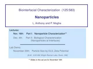
Biointerfacial Characterization (125:583) Nanoparticles L. Anthony and P. Moghe Lectures: Nov. 16th: Part I: Nanoparticle Characterization** Dec. 4th: Part II: Biological Characterization (Nanoparticles at Interfaces) Lab Demo: November 20th: Particle Size by DLS; Zeta Potential [8:40 - 9:20 AM; Wright-Rieman Labs, Room 396] ** Slides in this set are for November 16th
Outline for Nanoparticle Characterization: Part I • Introduction/context: Particles at biointerfaces Properties of particles in dispersions/emulsions • Particle Size and Particle Size Distribution • Surface Charge: Zeta Potential, Isoelectric Point, Electrophoretic Mobility Assigned papers • Nanoscale anionic macromolecules for selective retention of low-density lipoproteins • Chnari E, Lari HB, Tian L, Uhrich KE, Moghe PV • BIOMATERIALS 26 (17): 3749-3758 JUN 2005 Optimization of the preparation process for human serum albumin (HSA) nanoparticles K. Langer, S. Balthasar V. Vogel, N. Dinauer H. von Briesen D. Schubert INT. J. PHARMACEUTICS 257 (2003) 169-18
Other papers/information posted on class website: • Albumin-derived nanocarriers: Substrates for enhanced cell adhesive ligand display and cell motility • Sharma RI, Pereira M, Schwarzbauer JE, Moghe PV • BIOMATERIALS 27 (19): 3589-3598 JUL 2006 • Quantum dot bioconjugates for imaging, labeling, and sensing • Medintz, IL, Uyeda, HT, Goldman, ER, Mattoussi, H • NATURE MATERIALS, 4, 435-446 (2005) A Nanoparticle-Based Model Delivery System To Guide the Rational Design of Gene Delivery to the Liver. 1. Synthesis and Characterization Stephen R. Popielarski, Suzie H. Pun,† and Mark E. Davis* BIOCONJUGATE CHEM. 1063 2005, 16, 1063-1070 Vesicle Size Distributions Measured by Flow Field-Flow Fractionation Coupled with Multiangle Light Scattering Brian A. Korgel, John van Zanten, Harold Monbouquette BIOPHYSICAL JOURNAL 74 June 1998 3264–3272 • Short Monographs by Vendors: • Basic Principles of Particle Size Analysis • Zeta Potential, a Complete Course in Five Minutes • The Importance of Sample Viscosity in Dynamic Light Scattering Measurements • A Guide to Choosing a Particle Sizer
Outline for Part I: Nanoparticle Characterization • Introduction/context: Particles at biointerfaces Properties of particles in dispersions/emulsions • Particle Size and Particle Size Distribution • Surface Charge: Zeta Potential, Isoelectric Point, Electrophoretic Mobility
Introduction/Context: Particles at biointerfaces • Some reasons for using engineered nanoparticles in • biointerfacial research: • to study/effect a cellular process • Example:Albumin-derived nanocarriers: Substrates for • enhanced cell adhesive ligand display and cell motility • Sharma RI, Pereira M, Schwarzbauer JE, Moghe PV • BIOMATERIALS 27 (19): 3589-3598 JUL 2006 • to transport drugs/biomaterials or biomolecules • ***Example:Nanoscale anionic macromolecules for • selective retention of low-density lipoproteins • Chnari E, Lari HB, Tian L, Uhrich KE, Moghe PV • BIOMATERIALS 26 (17): 3749-3758 JUN 2005 • to visualize phenomena such as transport, sequestration, etc • Example: Quantum dot bioconjugates for • imaging, labeling, and sensing • Medintz, IL, Uyeda, HT, Goldman, ER, Mattoussi, H • NATURE MATERIALS, 4, 435-446 (2005) • *** Paper for discussion; examples given later in talk
Further modify/engineer particles/dispersion >Conjugated molecules >Buffers/salts >etc Make (or purchase) the nanoparticles and/or the dispersion Introduce particles into tissue/cellular/subcellular system and Study the particles and/or the effects of the particles tissue, cells or sub-cellular system under study Introduction/Context: Particles at biointerfaces Generic view of experiments with particles at biointerfaces:
Further modify/engineer particles/dispersion >Conjugated molecules >Buffers/salts >etc tissue, cells or sub-cellular system under study Introduction/Context: Properties of particles in dispersions/emulsions • Note: Properties of the particle at the biointerface depend on: • Intrinsic properties of particles AND • Mediating properties of the liquid phase(s) Introduce particles into tissue/cellular/subcellular system (in vitro usually) Study effect of particles Make (or purchase) the nanoparticles and/or dispersion Note: cellular milieu is a very complex dispersant!
tissue, cells or sub-cellular system under study Introduction/Context: Properties of particles in dispersions/emulsions Properties of Particles in dispersion or cellular milieu Average size (diameter) Size distribution Shape Bulk chemical composition Surface composition covalently linked molecules adsorbed species surface charge (zeta potential) Compliance/modulus, etc Pore size/roughness Crystalline/amorphous Refractive index Density Cover up Properties of Particles Average size (diameter) Size distribution Shape Bulk chemical composition Crystalline/amorphous Pore size/roughness Surface composition covalently linked molecules adsorbed species Compliance/modulus, etc Refractive index Density Properties of Dispersant (s) Aqueous or organic? (or mix?) Bulk composition Additives (what?, how much?) Ionic or non-charged Small molecules Bio and macro molecules pH, conductivity Viscosity Refractive index Density
tissue, cells or sub-cellular system under study Introduction/Context: Properties of particles in dispersions/emulsions Properties of Particles in dispersion or cellular milieu Average size (diameter) Size distribution Shape Bulk chemical composition Surface composition covalently linked molecules adsorbed species surface charge (zeta potential) Compliance/modulus, etc Pore size/roughness Crystalline/amorphous Refractive index Density Cover up Properties of Particles Average size (diameter) Size distribution Shape Bulk chemical composition Crystalline/amorphous Pore size/roughness Surface composition covalently linked molecules adsorbed species Compliance/modulus, etc Refractive index Density Properties of Dispersant (s) Aqueous or organic? (or mix?) Bulk composition Additives (what?, how much?) Ionic or non-charged Small molecules Bio and macro molecules pH, conductivity Viscosity Refractive index Density
Outline for Part I: Nanoparticle Characterization • Introduction/context: Particles at biointerfaces Properties of particles in dispersions/emulsions • Particle Size and Particle Size Distribution • Surface Charge: Zeta Potential, Isoelectric Point, Electrophoretic Mobility
ensemble fractionation counting/”sorting” Particle Size and Distribution: “Families” of Measurement Principles All particles analyzed simultaneously Based on first principles (optics, acoustics, etc) Size obtained from curve fitting/matrix inversion Distribution data from further computations on data Dynamic Light Scattering Static Light Scattering (& Laser Diffraction) Acoustic Attenuation Particles separated/sorted in space/time Based on differential (zonal) migration Size obtained by comparison with calibration standards Distribution data from detector output (graphical trace) Size Exclusion Chromatogr. Capillary Hydrodynamic Flow Field Flow Fractionation Electrophoresis [Sedimentation Velocity] Particles separated (diluted) but not sorted Based on size-dependent change in electronic (V, I, R, C, L) or optical signal Size obtained from prior calibration (instrumental) Distribution data from electronic “binning” of detector signals Coulter & Elzone (r) Accusizer (r) Microscopy with image analysis is analogous Also: hyphenated methods: e.g. fractionation method with ensemble-method detection (e.g. FFF-DLS).
Ensemble Methods Dynamic Light Scattering Brownian Motion of Particles; temporal fluctuations in intensity of scattered light Static Light Scattering (& Laser Diffraction) Angular dependence of intensity of scattered light (Rayleigh/Mie) (new, not widely used; not covered in this lecture) Acoustic Attenuation • “Instrument as black box” approach: • Put sample in cuvette (diluting if necessary per mfgr.’s instructions) • Enter known constants or accept instrument defaults (e.g. refractive index, viscosity, etc) • Choose adjustable parameters or accept instrument defaults • Press GO; come back when done; pick up print out Now, let’s take a closer look…
Dynamic Light Scattering (DLS) aka Photon Correlation Spectroscopy (PCS) aka Quasielastic Light Scattering (QELS) Step 1: Make the optical measurement: Temporal fluctuations in intensity of scattered light (wavelength and angle are set by instrument; RI is input or assumed) “speckle pattern” Figures from: http://www.science.uva.nl/~sprik/masterlaser/dlsexp/dls.html
Dynamic Light Scattering (DLS) aka Photon Correlation Spectroscopy (PCS) aka Quasielastic Light Scattering (QELS) Step 1: Make the optical measurement: Temporal fluctuations in intensity of scattered light (wavelength and angle are set by instrument; RI is input or assumed) **Step 2: Establish the correlation function and solve for Dr **Step 3: Use the Stokes-Einstein relationship to solve for Rh (Dh= 2Rh) **Step 4: Further process autocorrelation data to obtain distribution information **Done by the instrument, although user can adjust inputs and processing options
Dynamic Light Scattering (DLS) aka Photon Correlation Spectroscopy (PCS) aka Quasielastic Light Scattering (QELS) Step 1: Make the optical measurement: Temporal fluctuations in intensity of scattered light (wavelength and angle are set by instrument; RI is input or assumed) Step 2: Establish the correlation function and determine Dr Step 3: Use the Stokes-Einstein relationship to solve for Rh (Dh= 2Rh) Step 4: Further process autocorrelation data to obtain distribution information **Done by the instrument, although user can adjust inputs and processing options
Ensemble Methods Dynamic Light Scattering (DLS) aka Photon Correlation Spectroscopy (PCS) aka Quasielastic Light Scattering (QELS) Step 1: Make the optical measurement: Temporal fluctuations in intensity of scattered light (wavelength and angle are set by instrument; RI is input or assumed) Step 2: Establish the correlation function and determine Dr Step 3: Use the Stokes-Einstein relationship to solve for Rh (Dh= 2Rh) Step 4: Further process autocorrelation data to obtain distribution information The data reduction is done by the instrument, although user can adjust inputs and processing options
Ensemble Methods Static Light Scattering (and Laser Diffraction) Analogous to dynamic light scattering, but different optical property measured: Step 1:Measure the intensity of scattered light as a function of scattering angle for a dispersion of particles, usually at high dilution ** Step 2: Process the data to obtain the mean particle size and the distribution The data reduction is done by the instrument, although user can adjust inputs and processing options
Uncharged nanocarrier control COOH functionalized nanocarrier control LDL control Uncharged nanocarrers + LDL Charged nanocarrers + LDL COOH functionalized nanocarriers + LDL Example: Sizing of Nanoparticles with Dynamic Light Scattering:
Fractionation Methods Size Exclusion and other chromatography Capillary Hydrodynamic Flow Field Flow Fractionation (several variants) Capillary Electophoresis Sedimentation/Centrifugation • Instrument as black box approach: • Prepare sample if needed (diluted ; buffers and electrolytes added) • Prepare eluant and/or other media (gel, sucrose density gradient, etc) • Enter known constants or accept instrument defaults • Inject standard sample, start pump or rotor or turn on applied field • Run Calibration Standards, • Run Samples • Analyze data (graphically and mathematically) The details are not important, but note that fractionation is much more time and labor intensive than the ensemble methods. User must establish calibration curve Now, let’s take a closer look…
Fractionation Methods: Measurement Principles • Separation by differential (zonal) migration • Mixture in -------> Peaks 0ut • Carrier fluid pumped through column, channel, etc • Analye velocity is a characteristic fraction of carrier velocity, due to analyte interaction with (i) stationary phase in column • or (ii) to an applied field Xyz
Fractionation Methods: Measurement Principles Adsorption, partition, size exclusion Affinity, polarity,size Chromatography Electrophoretic mobility Ionic size, charge Electrophoresis Laminar flow profile (velocity gradient) Size (big first) Hydrodynamic flow Field-flow fractionation Laminar flow profile Particle mass Size (small first)
Example: Capillary Hydrodynamic Flow Comparison of CMP polishing slurries from two vendors Both slurrries nominally 50 nm particle size One is much more monodisperse than the other L.J. Anthony et al., Lucent Technologies, Bell Laboratories, unpublished work
Nanocarrier + LDL Nanocarrier LDL Example: Field Flow Fractionation Same system as in DLS example: nanocarriers for LDL sequestration (Data below are unpublished work; Chnari, Moghe et al. ) Note: this is also an example of Hyphenated Methods: Field Flow Fractionation with Static Light Scattering Detection Particles separated in time/space for “real” distribution; Accurate size data without calibration of FFF, just from the DLS
Example: Sedimentation Velocity Analysis Optimizing a process for preparing human serum albumin nanoparticles (from the assigned paper, K.Langer et al.) Assessing the process steps in particle synthesis and purification (note removal of fines) Assessing reproducibility of three identical runs
Caveat with all fractionation methods: Dispersion • Band-brodening in time: • later eluting zones are inherently broader • does not in itself reflect more polydispersity; • effects need to be deconvoluted to determine polydispersity
Counting/”Sorting” Methods AccuSizer (r) Coulter(r) and Elzone(r) Particle obscures a light bean transmitted through the cell; changes the light intensity Newer method; excellent down to ~ 300 nm, but true “nano” range still being optimized Particle displaces electrolyte in sampling cell; changes the signal across the electrodes Mature method, widely used - for cells and other “big” particles • “Instrument as black box” approach: • Put sample in reservoir (diluting if necessary per mfg. instructions • Enter known constants or accept instrument defaults (refractive index, viscosity, etc) • Choose adjustable parameters or accept instrument defaults • Press GO; come back when done; pick up print out Now, let’s take a closer look… http://openchemist.net/chemistry/coulter/node3.html
Counting/”Sorting” Methods: Measurement Principles After integration over the complete particle (i.e. over all the elements that contain the particle) we find that the instrument response is proportional to the volume ν of a spherical particle, modified by a function F: Function F can be found from the integration over the particle but other approaches, including a best fit from experimental results, are possible to find a proper equation for F. The following equation was found by De Blois and Bean using the experimental (best fit) approach: where d and D stand for the diameter of particle and orifice. Measurement is based on an experimentally determined relationship between “instrument response” and particle size http://openchemist.net/chemistry/coulter/node3.html
Examples: Counting/”Sorting” submicron particles (NiComp-PSS Accusizer) “Real world” data: Oversized (> 1 um) particles in chemical mechanical polishing process steps (silica slurry, 50 nm nominal particle size) Vendor’s data: Particles are ~245 and 380 nm As-received After polisher set-up After normal polishing run After wafer broke on pad http://www.shjnj.cn/CPJS-2.htm L.J. Anthony et al: Proc. 2nd Int. Symp. Chemical Planarization in Integrated Circuit Device Manufacturing, pp 181-196, The Electrochemical Society, 1998
Outline for Part I: Nanoparticle Characterization • Introduction/context: Particles at biointerfaces Properties of particles in dispersions/emulsions • Particle Size and Particle Size Distribution • Surface Charge: Zeta Potential, Isoelectric Point, Electrophoretic Mobility
Charged Species on Surfaces • Origins of Surface Charge • Characteristics of Surface Charge: Definitions • Zeta Potential and Electrophoretic Mobility • Determination of Zeta Potential • Zeta Potential vs pH • Assigned paper and other examples
Origins of Surface Charge Ionization of surface functional groups Organic/molecular: e.g. RCOOH <--> RCOO-, RNH2<--> RNH3+, etc As in protein/peptide C-terminus, N-terminus, certain side groups (aspartic acid, etc.) Note: can be intrinsic to the particle and/or surface- functionalized/derivatized (biotin, etc.) Inorganic/ionic: e.g. SiOH <> SiO-) (For example, glass beads, hydroxyapatite) 2) Adsorption of charged species Charged/ionizable molecules: e.g. surfactants, phospholipids (For example: SDS, constituents of ECM) Small ions: e.g. Ca++, Mg++, etc. (For example in certain physiological processes)
Characteristics of Surface Charge: Definitions Particle surface Stern Layer:Rigid layer of ions tightly bound to particle; ions travel with the particle Plane of hydrodynamic shear:Also called Slipping Plane:Boundary of the Stern layer: ions beyond the shear plane do not travel with the particle Diffuse Layer: Also called Electrical Double Layer: Ionic concentration not the same as in bulk; there is a gradient in concentration of ions outward from the particle until it matches the bulk
Characteristics of Surface Charge: Definitions Zeta potential: The electrical potential that exists at the slipping plane The magnitude of the zeta potential gives an indication of the potential stability of the colloidal system * If all the particles have a large zeta potential they will repel each other and there is dispersion stability * If the particles have low zeta potential values then there is no force to prevent the particles coming together and there is dispersion instability A dividing line between stable and unstable aqueous dispersions is generally taken at +30 or -30mV
+ - Zeta Potential and Electrophoretic Mobility In an applied electric field, charged particles travel toward the electrode of opposite charge. When attractive force of the electric field is balanced by the viscous drag on the particle, the particle travels with constant velocity. + - This velocity is the partlcle’s electrophoretic mobility, UE UE= 2zf(Ka)/3 Note relationship of zeta potential and electrophoretic mobility; therefore… Zeta potential can be determined by measuring UE z=Zeta potential =dielectric constant (of electrolyte) =dielectric constant (of electrolyte) f(Ka)= Henry’s function = ~1.5 (Smoluchowski approximation) for particles >~ 200 nm and electrolyte ~> 1 x 10⁻³ M = ~1.0 (Huckel approximation) for smaller particles and/or dilute/non-aqueous dispersions
Determination of Zeta Potential • Measure the Electrophoretic Mobility, UE (and know viscosity, dielectric constant; and choose a Henry function) • Solve Smoluchowski/Huckel Equation for Zeta Potential • Predominant Methods: • Laser Doppler Velocimetry • Phase Analysis Light Scattering (PALS) Method for particles with lower mobilities
Determination of Zeta Potential Principles of PALS: Similar to particle sizing by dynamic light scattering I.e. what is measured is temporal fluctuations in intensity of light scattered by the particles in the dispersion. In light scattering, the fluctuations are related to Brownian motion of particles. In PALS for ZP, the fluctuations are related to the movement of the particle in the applied field, i.e. to UE; The ZP is then calculated from the UE that is determined by the PALS measurement. (As in light scattering, the instrument’s autocorrelator and software take care of the data reduction.)
Zeta Potential vs pH pH dependency of ZP is very important! Remember, dispersion stability (or conversely, ability of particles to approach each other) is determined by ZP, with ~ 30 mV being the approximate cutoff. [In this example, the dispersion is stable below pH ~4 and above pH ~7.5] Typical plot of Zeta Potential vs pH. Zeta Potential, mV pH At ZP=0, net charge on particle is 0. This is called the isoelectric point
Zeta Potential and Electrolyte Concentration • Zeta potential also depends on electrolyte concentration! Remember that the ionic environment of the particle exists as a gradient that that eventually equilibrates with the bulk solution. • Too few ions: not enough charge to stabilize the particles • Too many ions: the double layer is compressed and the particles can approach (“salting out”)
Example: Zeta Potential Measurements Optimizing a process for preparing human serum albumin nanoparticles (from the assigned paper, K.Langer et al.) Zeta potential Particle diameter At low values of Zeta potential (near pH 6), the dispersion de-stabilizes and the particles agglomerate
Biointerfacial Characterization (125:583) Nanoparticles L. Anthony and P. Moghe Lectures: Nov. 16th: Part I: Nanoparticle Characterization** Dec. 4th: Part II: Biological Characterization (Nanoparticles at Interfaces) Lab Demo: November 20th: Particle Size by DLS; Zeta Potential [8:40 - 9:20 AM; Wright-Rieman Labs, Room 396] Coming attractions!