Introduction to Hidden Markov Models
330 likes | 803 Vues
Introduction to Hidden Markov Models. Markov Models. Set of states: Process moves from one state to another generating a sequence of states : Markov chain property: probability of each subsequent state depends only on what was the previous state:

Introduction to Hidden Markov Models
E N D
Presentation Transcript
Markov Models • Set of states: • Process moves from one state to another generating a sequence of states : • Markov chain property: probability of each subsequent state depends only on what was the previous state: • To define Markov model, the following probabilities have to be specified: transition probabilities and initial probabilities
Example of Markov Model 0.3 0.7 Rain Dry 0.2 0.8 • Two states : ‘Rain’ and ‘Dry’. • Transition probabilities: P(‘Rain’|‘Rain’)=0.3 , P(‘Dry’|‘Rain’)=0.7 , P(‘Rain’|‘Dry’)=0.2, P(‘Dry’|‘Dry’)=0.8 • Initial probabilities: say P(‘Rain’)=0.4 , P(‘Dry’)=0.6 .
Calculation of sequence probability • By Markov chain property, probability of state sequence can be found by the formula: • Suppose we want to calculate a probability of a sequence of states in our example, {‘Dry’,’Dry’,’Rain’,Rain’}. • P({‘Dry’,’Dry’,’Rain’,Rain’} ) = • P(‘Rain’|’Rain’) P(‘Rain’|’Dry’) P(‘Dry’|’Dry’) P(‘Dry’)= • = 0.3*0.2*0.8*0.6
Hidden Markov models. • Set of states: • Process moves from one state to another generating a sequence of states : • Markov chain property: probability of each subsequent state depends only on what was the previous state: • States are not visible, but each state randomly generates one of M observations (or visible states) • To define hidden Markov model, the following probabilities have to be specified: matrix of transition probabilities A=(aij), aij= P(si| sj) , matrix of observation probabilities B=(bi (vm )), bi(vm )= P(vm| si) and a vector of initial probabilities =(i), i= P(si) . Model is represented by M=(A, B, ).
Example of Hidden Markov Model 0.3 0.7 Low High 0.2 0.8 Rain 0.6 0.6 0.4 0.4 Dry
Example of Hidden Markov Model • Two states : ‘Low’ and ‘High’ atmospheric pressure. • Two observations : ‘Rain’ and ‘Dry’. • Transition probabilities: P(‘Low’|‘Low’)=0.3 , P(‘High’|‘Low’)=0.7 , P(‘Low’|‘High’)=0.2, P(‘High’|‘High’)=0.8 • Observation probabilities : P(‘Rain’|‘Low’)=0.6 , P(‘Dry’|‘Low’)=0.4 , P(‘Rain’|‘High’)=0.4 , P(‘Dry’|‘High’)=0.3 . • Initial probabilities: say P(‘Low’)=0.4 , P(‘High’)=0.6 .
Calculation of observation sequence probability • Suppose we want to calculate a probability of a sequence of observations in our example, {‘Dry’,’Rain’}. • Consider all possible hidden state sequences: • P({‘Dry’,’Rain’} ) = P({‘Dry’,’Rain’} , {‘Low’,’Low’}) + P({‘Dry’,’Rain’} , {‘Low’,’High’}) + P({‘Dry’,’Rain’} , {‘High’,’Low’}) + P({‘Dry’,’Rain’} , {‘High’,’High’}) • where first term is : • P({‘Dry’,’Rain’} , {‘Low’,’Low’})= • P({‘Dry’,’Rain’} | {‘Low’,’Low’}) P({‘Low’,’Low’}) = • P(‘Dry’|’Low’)P(‘Rain’|’Low’) P(‘Low’)P(‘Low’|’Low) • = 0.4*0.4*0.6*0.4*0.3
Main issues using HMMs : • Evaluation problem. Given the HMM M=(A, B, ) and the observation sequence O=o1 o2 ... oK , calculate the probability that model M has generated sequence O . • Decoding problem. Given the HMM M=(A, B, ) and the observation sequence O=o1 o2 ... oK , calculate the most likely sequence of hidden states si that produced this observation sequence O. • Learning problem. Given some training observation sequences O=o1 o2 ... oK and general structure of HMM (numbers of hidden and visible states), determine HMM parameters M=(A, B, ) that best fit training data. • O=o1...oK denotes a sequence of observations ok{v1,…,vM}.
Word recognition example(1). Amherst a 0.5 0.03 b A c 0.005 0.31 z • Typed word recognition, assume all characters are separated. • Character recognizer outputs probability of the image being particular character, P(image|character). Hidden state Observation
Word recognition example(2). • Hidden states of HMM = characters. • Observations = typed images of characters segmented from the image . Note that there is an infinite number of observations • Observation probabilities = character recognizer scores. • Transition probabilities will be defined differently in two subsequent models.
Word recognition example(3). m a m r t h e s Buffalo b u a o f f l A • If lexicon is given, we can construct separate HMM models for each lexicon word. Amherst 0.03 0.5 0.4 0.6 • Here recognition of word image is equivalent to the problem of evaluating few HMM models. • This is an application of Evaluation problem.
Word recognition example(4). a b v f o m r t h e s • We can construct a single HMM for all words. • Hidden states = all characters in the alphabet. • Transition probabilities and initial probabilities are calculated from language model. • Observations and observation probabilities are as before. • Here we have to determine the best sequence of hidden states, the one that most likely produced word image. • This is an application of Decoding problem.
Character recognition with HMM example. A • The structure of hidden states is chosen. • Observations are feature vectors extracted from vertical slices. • Probabilistic mapping from hidden state to feature vectors: 1. use mixture of Gaussian models • 2. Quantize feature vector space.
Exercise: character recognition with HMM(1) s1 s2 s3 A • HMM for character ‘A’ : • Transition probabilities: {aij}= • Observation probabilities: {bjk}= .8 .2 0 0 .8 .2 0 0 1 .9 .1 0 .1 .8 .1 .9 .1 0 • The structure of hidden states: • Observation = number of islands in the vertical slice. • HMM for character ‘B’ : • Transition probabilities: {aij}= • Observation probabilities: {bjk}= .8 .2 0 0 .8 .2 0 0 1 B .9 .1 0 0 .2 .8 .6 .4 0
Exercise: character recognition with HMM(2) • Suppose that after character image segmentation the following sequence of island numbers in 4 slices was observed: • { 1, 3, 2, 1} • What HMM is more likely to generate this observation sequence , HMM for ‘A’ or HMM for ‘B’ ?
Exercise: character recognition with HMM(3) • HMM for character ‘A’: • HMM for character ‘B’: Hidden state sequence Hidden state sequence Transition probabilities Transition probabilities Observation probabilities Observation probabilities s1 s1 s2s3 s1 s1 s2s3 .8 .2 .2 .9 0 .8 .9 = 0 .8 .2 .2 .9 0 .2 .6 = 0 s1 s2 s2s3 s1 s2 s2s3 .2 .8 .2 .9 .8 .2 .6 = 0.0027648 .2 .8 .2 .9 .1 .8 .9 = 0.0020736 s1 s2 s3s3 s1 s2 s3s3 .2 .2 1 .9 .8 .4 .6 = 0.006912 .2 .2 1 .9 .1 .1 .9 = 0.000324 Total = 0.0023976 Total = 0.0096768 Consider likelihood of generating given observation for each possible sequence of hidden states:
Evaluation Problem. • Evaluation problem. Given the HMM M=(A, B, ) and the observation sequence O=o1 o2 ... oK , calculate the probability that model M has generated sequence O . • Trying to find probability of observations O=o1 o2 ... oK by means of considering all hidden state sequences (as was done in example) is impractical: • NK hidden state sequences - exponential complexity. • Use Forward-Backward HMM algorithms for efficient calculations. • Define the forward variable k(i) as the joint probability of the partial observation sequence o1 o2 ... ok and that the hidden state at time k is si : k(i)= P(o1 o2 ... ok , qk=si)
Trellis representation of an HMM s1 sN s2 si sN s2 si s1 s1 s2 sj s1 s2 si sN sN o1 okok+1 oK = Observations a1j a2j aij aNj Time= 1 k k+1 K
Forward recursion for HMM • Initialization: • 1(i)= P(o1 , q1=si) = ibi (o1) , 1<=i<=N. • Forward recursion: • k+1(i)= P(o1 o2 ... ok+1 , qk+1=sj) = • iP(o1 o2 ... ok+1 , qk=si, qk+1=sj) = • iP(o1 o2 ... ok , qk=si) aij bj (ok+1 ) = • [i k(i) aij ] bj (ok+1 ) , 1<=j<=N, 1<=k<=K-1. • Termination: • P(o1 o2 ... oK) = iP(o1 o2 ... oK , qK=si) = i K(i) • Complexity : • N2K operations.
Backward recursion for HMM • Define the forward variable k(i) as the joint probability of the partial observation sequence ok+1 ok+2 ... oK given that the hidden state at time k is si : k(i)= P(ok+1 ok+2 ... oK |qk=si) • Initialization: • K(i)= 1 , 1<=i<=N. • Backward recursion: • k(j)= P(ok+1 ok+2 ... oK |qk=sj) = • iP(ok+1 ok+2 ... oK , qk+1=si|qk=sj) = • iP(ok+2 ok+3 ... oK |qk+1=si) aji bi (ok+1 ) = • i k+1(i) aji bi (ok+1 ) , 1<=j<=N, 1<=k<=K-1. • Termination: • P(o1 o2 ... oK) = iP(o1 o2 ... oK , q1=si) = • iP(o1 o2 ... oK |q1=si) P(q1=si) = i 1(i) bi (o1) i
Decoding problem • Decoding problem. Given the HMM M=(A, B, ) and the observation sequence O=o1 o2 ... oK , calculate the most likely sequence of hidden states si that produced this observation sequence. • We want to find the state sequence Q= q1…qK which maximizes P(Q | o1 o2 ... oK ) , or equivalently P(Q , o1 o2 ... oK ) . • Brute force consideration of all paths takes exponential time. Use efficient Viterbi algorithm instead. • Define variable k(i) as the maximum probability of producing observation sequence o1 o2 ... ok when moving along any hidden state sequence q1… qk-1 and getting into qk= si . • k(i) = max P(q1… qk-1 ,qk= si,o1 o2 ... ok) • where max is taken over all possible paths q1… qk-1 .
Viterbi algorithm (1) s1 si sN sj qk-1 qk a1j aij aNj • General idea: • if best path ending in qk= sjgoes through qk-1= sithen it should coincide with best path ending in qk-1= si. • k(i) = max P(q1… qk-1 ,qk= sj,o1 o2 ... ok) = • maxi [ aij bj (ok ) max P(q1… qk-1= si,o1 o2 ... ok-1) ] • To backtrack best path keep info that predecessor of sj was si.
Viterbi algorithm (2) • Initialization: • 1(i) = max P(q1= si,o1) = ibi (o1) , 1<=i<=N. • Forward recursion: • k(j) = max P(q1… qk-1 ,qk= sj,o1 o2 ... ok) = • maxi [ aij bj (ok ) max P(q1… qk-1= si,o1 o2 ... ok-1) ]= • maxi [ aij bj (ok ) k-1(i) ] , 1<=j<=N, 2<=k<=K. • Termination: choose best path ending at time K • maxi [ K(i) ] • Backtrack best path. This algorithm is similar to the forward recursion of evaluation problem, with replaced by max and additional backtracking.
Learning problem (1) • Learning problem. Given some training observation sequences O=o1 o2 ... oK and general structure of HMM (numbers of hidden and visible states), determine HMM parameters M=(A, B, ) that best fit training data, that is maximizes P(O |M) . • There is no algorithm producing optimal parameter values. • Use iterative expectation-maximization algorithm to find local maximum of P(O |M) - Baum-Welch algorithm.
Learning problem (2) Number of times observation vm occurs in state si Number of times in state si bi(vm )= P(vm| si)= • If training data has information about sequence of hidden states (as in word recognition example), then use maximum likelihood estimation of parameters: • aij= P(si| sj) = Number of transitions from state sj to state si Number of transitions out of state sj
Baum-Welch algorithm aij= P(si| sj) = Expected number of transitions from statesjto statesi Expected number of transitions out of statesj Expected number of times observationvmoccurs in statesi Expected number of times in statesi bi(vm )= P(vm| si)= i = P(si) = Expected frequency in statesiat time k=1. General idea:
Baum-Welch algorithm: expectation step(1) • Define variable k(i,j) as the probability of being in state si at time k and in state sj at time k+1, given the observation sequence o1 o2 ... oK . • k(i,j)= P(qk= si,qk+1= sj|o1 o2 ... oK) P(qk= si,qk+1= sj,o1 o2 ... ok) P(o1 o2 ... ok) k(i,j)= = P(qk= si,o1 o2 ... ok) aij bj (ok+1 ) P(ok+2 ... oK |qk+1= sj) P(o1 o2 ... ok) = k(i)aij bj (ok+1 )k+1(j) i jk(i)aij bj (ok+1 )k+1(j)
Baum-Welch algorithm: expectation step(2) k(i)k(i) i k(i)k(i) P(qk= si,o1 o2 ... ok) P(o1 o2 ... ok) k(i)= = • Define variable k(i) as the probability of being in state si at time k, given the observation sequence o1 o2 ... oK . • k(i)= P(qk= si|o1 o2 ... oK)
Baum-Welch algorithm: expectation step(3) • We calculated k(i,j) = P(qk= si,qk+1= sj|o1 o2 ... oK) • and k(i)= P(qk= si|o1 o2 ... oK) • Expected number of transitions from state si to state sj = • = k k(i,j) • Expected number of transitions out of state si = k k(i) • Expected number of times observation vm occurs in state si = • = k k(i) , k is such that ok= vm • Expected frequency in state siat time k=1 : 1(i) .
Baum-Welch algorithm: maximization step k k(i,j) k k(i) = Expected number of transitions from statesjto statesi Expected number of transitions out of statesj aij = k k(i,j) k,ok= vmk(i) Expected number of times observation vmoccurs in state si Expected number of times in state si bi(vm )= = i = (Expected frequency in statesiat time k=1) =1(i).
