Epidemics on networks
Epidemics on networks. Lorenzo Pellis. University of Warwick, UK Warwick, 22 nd September 2016. Basic SIR and SIS Key epidemiological quantities Relaxing basic assumptions. Introduction. Basic SIR and SIS Key epidemiological quantities Relaxing basic assumptions. Introduction.

Epidemics on networks
E N D
Presentation Transcript
Epidemics on networks Lorenzo Pellis University of Warwick, UK Warwick, 22nd September 2016
Basic SIR and SIS Key epidemiological quantities Relaxing basic assumptions Introduction
Basic SIR and SIS Key epidemiological quantities Relaxing basic assumptions Introduction
Framework • SIR epidemic model • Large population • Single initial case • Rest of the population is fully susceptible Examples: • Influenza pandemics • SARS • Ebola S I R
The equations Equations: • Assumptions: • Homogeneous mixing • Constant recovering rate • Many possible variations on the same theme… Initial conditions: Parameters:
Alternative framework • SISepidemic model • Large population • Single initial case • Rest of the population is fully susceptible Examples: • Chlamydia • Human papilloma virus • (Respiratorysyncytial virus / influenza) S I
The equations Equations: • Assumptions: • Homogeneous mixing • Constant recovering rate • Many possible variations on the same theme… Initial conditions: Parameters:
Other possible frameworks • Single epidemic wave: • SIR • SEIR • SITR • MSEIR • … • Endemic equilibrium: • SIS • SEIS • SIRS • SIR with demography • …
Basic SIR and SIS Key epidemiological quantities Relaxing basic assumptions Introduction
Key epidemiological quantities Can we provide summary information of the full dynamics? • Real-time growth rate • Thresholdcondition • Epidemicfinal size • ...
Key epidemiological quantities Can we provide summary information of the full dynamics? • Real-time growth rate • Thresholdcondition • Epidemicfinal size • ...
The equations Equations: • Assumptions: • Homogeneous mixing • Constant recovering rate • Many possible variations on the same theme… Initial conditions: Parameters:
Linear SIR: Malthusian growth • If , at the beginning the number of cases increases exponentially, with exponent • If , the number of cases decreases and the epidemic “dies out” • is called Malthusian parameter, or real-time growth rate
Key epidemiological quantities Can we provide summary information of the full dynamics? • Real-time growth rate • Threshold condition • Epidemic final size • ...
Threshold condition • A large epidemic occurs if and only if • For roughly 50 years, the same condition was expressed by mathematicians as where was called relative removal rate • During the ’80s (HIV epidemic), biologists and epidemiologists stepped in, interpreting it as: • Clearly it is the same thing, but...
Basic reproduction number R0 • Called basic reproduction number • Defined as the average number of new cases, generated by a single case, throughout the infectious period, in a totally susceptible population • An epidemic occurs if and only if Average number of new cases generate by a single case, per unit of time, in a totally susceptible population = = Average duration of the infectious period
Key epidemiological quantities Can we provide summary information of the full dynamics? • Real-time growth rate • Threshold condition • Epidemic final size • ...
Epidemic final size • Largest solution of
Properties of R0 • Threshold parameter: • If , only small epidemics • If , only large epidemics
Properties of R0 • Threshold parameter: • If , only small epidemics • If , only large epidemics • Average final size:
Properties of R0 • Threshold parameter: • If , only small epidemics • If , only large epidemics • Average final size: • Critical vaccination coverage:
Properties of R0 • Threshold parameter: • If , only small epidemics • If , only large epidemics • Average final size: • Critical vaccination coverage:
Basic SIR and SIS Key epidemiological quantities Relaxing basic assumptions Introduction
Relaxing assumptions • Deterministic model: • Make it stochastic • Constant infectivity and recovery rate: • Constant infectivity, any duration of infectious period • Time-varying infectivity • Homogeneous mixing: • Heterogeneous mixing • Households models • Network models
Relaxing assumptions • Deterministic model: • Make it stochastic • Constant infectivity and recovery rate: • Constant infectivity, any duration of infectious period • Time-varying infectivity • Homogeneous mixing: • Heterogeneous mixing • Households models • Network models
Markovian stochastic SIRmodel • Population of individuals • Upon infection, each case : • remains infectious for a duration , , • makes infectious contacts with each person in the population at the points of a homogeneous Poisson process with rate • Contacted individuals, if susceptible, become infected • Recovered individuals are immune to further infection
Effects of stochasticity • Random delays • But when the epidemic takes off, a deterministic approximation is very reasonable (CLT) • Early extinction
Branching process approximation • Follow the epidemic in generations: • number of infected cases in generation (pop. size ) • For every fixed , where is the -th generation of a simple Galton-Watson branching process (BP) • Let be the random number of children of an individual in the BP, and let be the offspring distribution. • Define • We have “linearised” the early phase of the epidemic • Pellis, Ball & Trapman(2012)
Properties of R0 - deterministic • Threshold parameter: • If , only small epidemics • If , only large epidemics • Average final size: • Critical vaccination coverage:
Properties of R0 - stochastic • Threshold parameter: • If , only small epidemics • If , possible large epidemics • Average final size (cond on non-extinct): • Critical vaccination coverage:
Relaxing assumptions • Deterministic model: • Make it stochastic • Constant infectivity and recovery rate: • Constant infectivity, any duration of infectious period • Time-varying infectivity • Homogeneous mixing: • Heterogeneous mixing • Households models • Network models
Standard stochastic SIR model (sSIR) • Population of individuals • Upon infection, each case : • remains infectious for a duration , iid • makes infectious contacts with each person in the population at the points of a homogeneous Poisson process with rate • Contacted individuals, if susceptible, become infected • Recovered individuals are immune to further infection • Even more realistic:
Relaxing assumptions • Deterministic model: • Make it stochastic • Constant infectivity and recovery rate: • Constant infectivity, any duration of infectious period • Time-varying infectivity • Homogeneous mixing: • Heterogeneous mixing • Households models • Network models
Multitype epidemic model • Different types of individuals • Define the next generation matrix (NGM): where is the average number of type- cases generated by a type- case, throughout the entire infectious period, in a fully susceptible population Properties of the NGM: • Non-negative elements • We assume positive regularity
Basic reproduction number R0 Naïve definition: “ Average number of new cases generated by a typical case, throughout the entire infectious period, in a large and otherwise fully susceptible population ” What is a typical case? What do we mean by fully susceptible population?
Multitype epidemic model • Different types of individuals • Define the next generation matrix (NGM): where is the average number of type- cases generated by a type- case, throughout the entire infectious period, in a fully susceptible population Properties of the NGM: • Non-negative elements • We assume positive regularity
Perron-Frobenius theory • Single dominant eigenvalue , which is positive and real • “Dominant” eigenvector has non-negative components • For every starting condition, after a few generations, the proportions of cases of each type in a generation converge to the components of the dominant eigenvector , with per-generation multiplicative factor
First few generations where
Perron-Frobenius theory • Single dominant eigenvalue , which is positive and real • “Dominant” eigenvector has non-negative components • For every starting condition, after a few generations, the proportions of cases of each type in a generation converge to the components of the dominant eigenvector , with per-generation multiplicative factor • Define • Interpret “typical” case as a linear combination of cases of each type given by
Relaxing assumptions • Deterministic model: • Make it stochastic • Constant infectivity and recovery rate: • Constant infectivity, any duration of infectious period • Time-varying infectivity • Homogeneous mixing: • Heterogeneous mixing • Households models • Network models
Model illustration • Pellis, Ferguson & Fraser (2009)
Household reproduction number R* • Consider a within-household epidemic started by one initial case • Define: • average household final size, excluding the initial case • average number of global infections an individual makes • “Linearise” the epidemic process at the level of households: • Pellis, Ball & Trapman(2012)
Household reproduction number R* • Consider a within-household epidemic started by one initial case • Define: • average household final size, excluding the initial case • average number of global infections an individual makes • “Linearise” the epidemic process at the level of households: • Pellis, Ball & Trapman(2012)
Relaxing assumptions • Deterministic model: • Make it stochastic • Constant infectivity and recovery rate: • Constant infectivity, any duration of infectious period • Time-varying infectivity • Homogeneous mixing: • Heterogeneous mixing • Households models • Network models
Basic concepts • What is a network? • A pair (set of nodes, set of edges) • Can be represented with an adjacency matrix • What does it represent? • Anything that involves actors and actor-actor interactions • Nodes can be individuals, groups, households, cities, locations… • Edges can be transmissions, friendships, flights routes… • Some properties: • Degree distribution • Assortativity (degree correlation) • Clustering • Modularity • Betweenness centrality
Constructing a network • Just draw one • Direct measurement • Deterministic algorithm • Stochastic algorithm • Erdös-Rényi random graph • Configuration model • Preferential attachment model (e.g. BA model scale-free) • Small world network • A random graph: • is a family of graphs, specified by a random algorithm • each specific graph occurs with a certain probability • its properties are random variables (e.g. size of the largest connected component) or mean/variance of such variables
Epidemics on a network • Some networks are labelled (e.g. age of nodes) • In an epidemic, labels vary over time (e.g. S, I, R) • If you run a stochastic epidemic on a random graph, results are random because of the epidemic process AND of the graph • Usually one thinks: but there might be better approaches: • making the graph as the epidemic is running • if possible, average over the graph family and only then over the epidemic process • …