EEGS Short Course Processing of Seismic Refraction Tomography Data
760 likes | 2.37k Vues
EEGS Short Course Processing of Seismic Refraction Tomography Data. SAGEEP 2010 Keystone, Colorado April 10, 2010. Instructors. Schedule. 13:00 – 13:10 Overview and introductions 13:10 – 13:40 Introduction to refraction method & Rayfract®

EEGS Short Course Processing of Seismic Refraction Tomography Data
E N D
Presentation Transcript
EEGS Short CourseProcessing of Seismic Refraction Tomography Data SAGEEP 2010 Keystone, Colorado April 10, 2010
Schedule 13:00 – 13:10 Overview and introductions 13:10 – 13:40 Introduction to refraction method & Rayfract® 13:40 – 14:40 Rayfract® tutorial dataset #1: Val de Travers 14:40 – 14:55 Break 14:55 – 15:45 Rayfract® tutorial dataset #2: Success Dam 15:45 – 17:00 Work on individual datasets
Smooth Inversion = 1D gradient initial model +2D WET Wavepath Eikonal Traveltime tomography Get minimum-structure 1D gradient initial model : Top : pseudo-2D Delta-t-V display • 1D Delta-t-V velocity-depth profile below each station • 1D Newton search for each layer • velocity too low below anticlines • velocity too high below synclines • based on synthetic times for Broad Epikarst model (Sheehan, 2005a, Fig. 1). Bottom : 1D-gradient initial model • generated from top by lateral averaging of velocities • minimum-structure initial model • Delta-t-V artefacts are completely removed
2D WET Wavepath Eikonal Traveltime inversion • rays that arrive within half period of fastest ray : tSP + tPR – tSR <= 1 / 2f (Sheehan, 2005a, Fig. 2) • nonlinear 2D optimization with steepest descent, to determine model update for one wavepath • SIRT-like back-projection step, along wave paths instead of rays • natural WET smoothing with wave paths (Schuster 1993, Watanabe 1999) • partial modeling of finite frequency wave propagation • partial modeling of diffraction, around low-velocity areas • WET parameters sometimes need to be adjusted, to avoid artefacts • see RAYFRACT.HLP help file Fresnel volume or wave path approach :
Supported Recording Geometries Compressional (P-) wave & shear (S-) wave interpretation • Surface refraction, see appended tutorials • Crosshole tomography, see IGTA13.PDF • Multi-offset VSP, see WALKAWAY.PDF • Zero-offset downhole VSP, see VSP.PDF • Combine downhole shots with crosshole shots, if all receivers in same borehole, for all shots • POISSON.PDF: determine dynamic Poisson’s Ratio from P & S wave
Supported Recording Geometries (cont.) Constrain surface refraction interpretation with uphole shots • See COFFEY04.PDF. Use 1D-gradient initial model or constant-velocity • Anisotropy: velocity may be dependent on predominant direction of ray and wave path propagation. This becomes visible directly adjacent to borehole. Imaged structure/layering is blurred out. • Velocity inversions / low-velocity layers may become visible • Walkaway VSP shots recorded with one or more boreholes may be converted to uphole shots by resorting traces by common receiver. Then import these exported uphole shots into one surface refraction profile. • Use two or more boreholes for improved resolution and reliability
Survey Design Requirements and Suggestions • Survey requirements • 24 or more channels/receivers per shot recommended • WET works with shots recorded only in one direction • more reliable with shots recorded in both directions and reciprocal shots. This enables correction of picking errors. • at least 1 shot every 3 receivers, ideally every 2 receivers • Survey design suggestions • overlapping receiver spreads, so internal far offset shots can be used for WET tomography. • receiver spreads should overlap by 30% to 50%. • see OVERLAP.PDF and RAYFRACT.PDF chapter Overlapping receiver spreads, on your CD
Station Numbering Concept • Single station spacing defined for each profile • Typically equivalent to receiver spacing • All receivers at integer station numbers • Shot locations can be fractional station numbers • Station spacing = greatest common divisor of all receiver spacings across profile • Example: Rx position (ft/m) = 0, 5, 15, 25, 45, 50, 60,... Station spacing = 5 (ft/m) Rx position (station numbers) = 0, 1, 3, 5, 9, 10, 12,... • See Defining your own layout types in Rayfract® Help|Contents
Irregular Receiver Spread Types Supported • Several standard receiver spread types already defined in Rayfract® • For input file formats SEG-2 and ASCII column format, you always need to define an irregular receiver spread type, even in case of missing channels e.g. at road crossing. • For all other input file formats e.g. Interpex Gremix™, Geometrics SeisImager™ and OPTIM LLC SeisOpt® , you don’t need to define your own spread type if the spread layout used is regular, with constant channel separation (receiver spacing), and some channels missing e.g. due to road crossing. • The default spread layout type “10: 360 channels” will work fine in this case. The number of active channels used is recognized automatically by our import routine. • See Receiver spread types in Rayfract® Help|Contents
First Break Picks Reflections/diffractions from cavity? ? ? Where to pick first breaks? • Real dataset over cavity • Raw data – no filtering ? ?
First Break Picks Artifact of HP filtering Where to pick first breaks? • Same real dataset over cavity • High-pass filter applied • Caution: Wavelet precursor results ? ? ? Air Wave
First Break Picks - Synthetic Cavity Data Easy First Arrival Picking!
First Break Picks - Messy Real Cavity Data Messy Area for picking
Generalized Rayfract® Flow Chart Create new profile database Define header information (minimum: Line ID, Job ID, instrument, station spacing (m)) Import data (ASCII first break picks or shot records) Update geometry information (shot & receiver positional information) Run inversion Smooth invert|WET with 1D-gradient initial model (results output in Golden Software’s Surfer) Edit WET & 1D-gradient parameters & settings
Smooth Inversion, DeltatV and WET Parameters • always start with default parameters: run Smooth inversion without changing any setting or parameter • next adapt parameters and option settings if required, e.g. to remove artefacts or increase resolution • more smoothing and wider WET wavepath width in general results in less artefacts • increasing the WET iteration count generally improves resolution • don’t over-interpret data if uncertain picks : use more smoothing and/or wider wavepaths. • explain traveltimes with minimum-structure model • tuning of parameters and settings may introduce or remove artefacts. Be ready to go one step backwards. • use Wavefront refraction method (Ali Ak, 1990) for independent velocity estimate.
Smooth inversion options in Settings submenu to vary the 1D-gradient initial model
Delta-t-V Options in Settings submenu to vary the 1D-gradient initial model
Tutorial #1Val de Travers, Switzerland, GeoExpert agP-wave surface profile29 shots, 48 traces per shot, roll-along recording with overlapping receiver spreadsReceiver spacing = 5mPlanning of a highway tunnel in an area prone to rockfalls, in Jura Mountains north of Geneva and near French border
Create new profile • Start up Rayfract® software with desktop icon or Start menu • 2 Select File|New Profile… • 3 Set File name to TRA9002 and click Save
Fill in profile header • 1 Select Header|Profile… Use function key F1 for help on fields. • Set Line ID to TRA9002 and Job ID to Tutorial • Set Instrument to Bison-2 9000 and Station spacing to 5m • Hit ENTER, and confirm the prompt
Seismic data import • Download and unzip http://rayfract.com/tutorials/TRA9002.ZIP to • directory C:\RAY32\TUTORIAL • 2 Select File|Import Data… for Import shots dialog, see above • 3 Set Import data type to Bison-2 9000 Series • 4 Click Select button, select file TRAV0201 in directory C:\RAY32\TUTORIAL • 5 Click on Open, Import shots, and confirm the prompt
Import each shot Click on Read for all shots shown in Import Shot dialog, see above. Don’t change Layout start and Shot pos., these are correct already
Update geometry and first breaks 1 Select File|Update header data|Update Station Coordinates… 2 Click on Select and C:\RAY32\TUTORIAL\TRA9002.COR 3 Click on Open, Import File and confirm the prompt 4 Select File|Update header data|Update First Breaks and C:\RAY32\TUTORIAL\TRA9002.LST and click Open
View and repick traces, display traveltime curves • 1 Select Trace|Shot gather and Window|Tile. Browse shots with F7/F8 • 2 Click on Shot breaks window and press ALT-P • 3 Set Maximum time to 130 msecs. and hit ENTER • 4 Click on Shot traces window and press F1 twice to zoom time • CTRL-F1 twice to zoom amplitude, CTRL-F3 twice to toggle trace fill mode • Select Processing|Color traces and Processing|Color trace outline • Use up/down/left/right arrow keys to navigate along and between traces • Zoom spread with SHIFT-F1. Pan zoomed sections with SHIFT-PgDn/PgUp • Optionally repick trace with left mouse key or space bar, delete first break with ALT-DEL or SHIFT-left mouse key. Press ALT-Y to redisplay traveltime curves
Smooth inversion of first breaks : 1D-gradient initial model 1 Select Smooth invert|WET with 1D-gradient initial model 2 Once the 1D-gradient model is shown in Surfer™, click on Rayfract® icon at bottom of screen, to continue. Confirm following prompts.
Smooth inversion of first breaks : 2D WET tomography • Click on Surfer icon shown at bottom of screen • Select View|Object Manager to show outline at left, if not yet shown • Click on Image in outline, right-select Properties. • Click on Colors spectrum, adjust Minimum and/or Maximum fields.
Display modeled picks and traveltime curves • Click on Rayfract® icon at bottom of screen • Select Refractor|Shot breaks to view picked and modeled (blue) times • Press F7/F8 keys to browse through shot-sorted traveltime curve • Use Mapping|Gray picked traveltime curves to toggle curve pen style
Display WET wavepath coverage 1 Click on Surfer icon at bottom of screen 2 Use CTRL-TAB to cycle between WET tomogram, wavepath coverage plot and 1D-gradient initial model
Optionally increase number of WET iterations • Click on Rayfract® icon at bottom of screen • Select WET Tomo|Interactive WET tomography… • Change Number of WET tomography iterations to 100 • Click button Start tomography processing, confirm prompts as above
Tutorial #2Success Dam, Porterville, CA, USGSP-wave surface profile48 shots into 48 fixed geophonesstation spacing = 15ftDetermine depth to bedrock, likelihood of liquefiable zones, define lateral continuity of geologic units, and identify faults/fracture zones
Create new profile • Start up Rayfract® software with desktop icon or Start menu • Select File|New Profile… • 3 Set File name to LINE3P and click Save
Fill in profile header • 1 Select Header|Profile… Use function key F1 for help on fields. • Set Line ID to LINE3P and Job ID to Success Dam Tutorial • Set Instrument to unknown and Station spacing to 5m • Hit ENTER, and confirm the prompt
Seismic data import • Unzip http://rayfract.com/tutorials/LINE3P.ZIP to C:\RAY32\SUCCESS • Select File|Import Data… for Import shots dialog, see above • Set Import data type to SEG-2 • Click Select button, set Files of type to ABEM files (*.SG2) • Select file USGS01.SG2 in directory C:\RAY32\SUCCESS • Click on Open, Import shots, and confirm the prompt
Import each shot Click on Read for all shots shown in Import Shot dialog, see above. Don’t change Layout start and Shot pos., these are correct already
Update geometry and first breaks 1 Select File|Update header data|Update Station Coordinates… 2 Click on Select and C:\RAY32\SUCCESS\COORDS.COR 3 Click on Open, Import File and confirm the prompt 4 Select File|Update header data|Update Shotpoint coordinates… 5 Select C:\RAY32\SUCCESS\SHOTPTS.SHO, click Open, confirm prompt 6 Select File|Update header data|Update First Breaks and C:\RAY32\SUCCESS\BREAKS.LST and click Open
View and zoom traces, display traveltime curves • 1 Select Trace|Shot gather and Window|Tile. Browse shots with F7/F8 • 2 Click on Shot breaks window and select Mapping|Gray picked traveltime curves • 3 Press ALT-P, set Maximum time to 90 msecs. and hit ENTER • 4 Click on Shot traces window and press F1 twice to zoom time • 5 CTRL-F1 four times to zoom amplitude, CTRL-F3 twice to toggle trace fill mode • 6 Select Processing|Color traces and Processing|Color trace outline • Use up/down/left/right arrow keys to navigate along and between traces • Zoom spread with SHIFT-F1. Pan zoomed sections with SHIFT-PgDn/PgUp
Smooth inversion of first breaks : 1D-gradient initial model 1 Select Smooth invert|WET with 1D-gradient initial model 2 Once the 1D-gradient model is shown in Surfer™, click on Rayfract® icon at bottom of screen, to continue. Confirm following prompts.
Smooth inversion of first breaks : 2D WET tomography • Click on Surfer® icon shown at bottom of screen • Select View|Object Manager to show outline at left, if not yet shown • Click on Image in outline, right-select Properties. • Click on Colors spectrum, adjust Minimum and/or Maximum fields.
Display WET wavepath coverage • 1 Click on Surfer® icon at bottom of screen • Use CTRL-TAB to cycle between WET tomogram, wavepath coverage plot and 1D-gradient initial model
Display modeled picks and traveltime curves • Click on Rayfract® icon at bottom of screen • Select Refractor|Shot breaks to view picked and modeled (blue) times • Press F7/F8 keys to browse through shot-sorted traveltime curve • Use Mapping|Gray picked traveltime curves to toggle curve pen style
Increase WET iteration count to improve resolution • Select WET Tomo|Interactive WET tomography… • Click button Reset to reset WET parameters to default settings • Change Number of WET tomography iterations to 100 • Click button Start tomography processing, confirm prompts as above • 5 Note improved imaging of fault : velocity step in center of tomogram
Flip over tomogram • Select Grid|Turn around grid file by 180 degrees… • Select file C:\RAY32\GRADTOMO\VELOIT100.GRD, click Open • Select Grid|Image and contour velocity and coverage grids… • 4 Select file C:\RAY32\GRADTOMO\VELOIT100.GRD, click Open • 5 Click on Surfer icon at bottom of screen, use CTRL-TAB to cycle