Download
1 / 33
410 likes | 735 Vues
Seismic Refraction Exercise for a Hydrogeology Course. Devin Castendyk State University of New York, College at Oneonta. Basic hydrogeologic questions. How deep is the water table? What is the stratigraphy below a site?. Traditional solution:. Drill several boreholes & install wells:

E N D
Seismic Refraction Exercise for a Hydrogeology Course Devin Castendyk State University of New York, College at Oneonta
Basic hydrogeologic questions • How deep is the water table? • What is the stratigraphy below a site?
Traditional solution: Drill several boreholes & install wells: Expensive ($500-$2000 per well) Labor Intensive Time If site is contaminated: Disposal of contaminated core Clean equipment
What students need to know • What are seismic waves? • Useful property: Waves travel at different velocities • True of different phases (e.g. solid, liquid, and gas) • True of different Earth materials: • Dry soil (vadose zone) ~ 1000 ft/sec • Wet soil (phreatic zone)~ 5000 ft/sec • Shale = 7000-9000 ft/sec • Sandstone = 8000-12,000 ft/sec • Granite > 17,000 ft/sec • If we can measure the velocity of seismic waves versus depth, we can define the water table and infer the stratigraphy at depth without intrusive methods.
Objective: Depth Velocity Interpretation 0-10 ft 1000 ft/sec Unsaturated Soil Water Table 10-20 ft 5000 ft/sec Saturated Soil > 20 ft 12,000 ft/sec Bedrock
How to measure the composition of a 1-layer, homogeneous site • Place a geophone (mini-seismometer) at a known distance from a seismic source • Generate a seismic wave • Measure the time it takes the P-Wave to move from the source to the geophone • Calculate and interpret the velocity:
How to address 2-layered site using seismic refraction • Step 1: Use multiple geophones (an array) typically spaced equal distances apart (e.g. 10 feet) • Step 2: Generate a seismic wave • Interpret results
Set up the geophone array Geophone
“Bison Digital Instantaneous Floating Point Signal Stacking Seismograph”
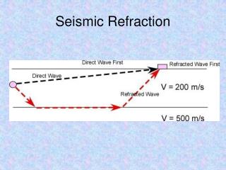
How seismic waves refract • Time 1: • Direct wave travels in all directions from source • Vibrations from Layer 1 arrive at closest geophone (1) 10 9 1 2 3 4 5 6 7 8 Soil Bedrock
How seismic waves refract • Time 2: • Wave front reaches layer boundary • Vibrations from Layer 1 recorded by next closest geophone (2) 10 9 1 2 3 4 5 6 7 8 Soil Bedrock
How seismic waves refract • Time 3: • Wave front travels faster through Layer 2 (bedrock) than Layer 1 (soil). • This causes the interface between the layers to vibrate in advance of the wave front in Layer 1 (seismic refraction). • Waves generated by the interface travel back to surface. 10 9 1 2 3 4 5 6 7 8 Soil Refracted Wave Bedrock
How seismic waves refract • Time 4: • Refracted waves reach geophones ahead of direct waves from source. 10 9 1 2 3 4 5 6 7 8 Soil Refracted Wave Bedrock
Raw data Seismic Refraction, SUNY Oneonta, May 2006 Geophone Number P-Wave Arrival Time (milliseconds)
Data analysis Step 1: Pick P-Wave arrival times (first deviation) Step 2: Graph arrival time versus distance
Pit P-wave arrival times Seismic Refraction, SUNY Oneonta, May 2006 Geophone Number P-Wave Arrival Time (milliseconds)
P-wave velocity calculations Step 3: Connect points corresponding to the same velocity Step 4: Calculate the velocity represented by each line
v2=5000 ft/sec v1=1000 ft/sec v3=12,000 ft/sec
Depth of boundary between Layer 1 and Layer 2 • Step 5: Calculate the depth of the interface between Layer 1 and Layer 2. The depth (z1) from the surface to the first interface is calculated using the following equation: Where Xc1 is the distance to the first intersecting velocity lines. This represents the distance from the source where the direct wave and the refracted wave arrive at the same time.
v2=5000 ft/sec v1=1000 ft/sec v3=12,000 ft/sec Xc = 20 feet
Depth of boundary between Layer 2 and Layer 3 • Step 6: Calculate the depth of the interface between Layer 2 and Layer 3. The depth (z2) from the surface to the first interface is calculated using the following equation: Where Xc2 is the distance to the first intersecting velocity lines.
v2=5000 ft/sec v1=1000 ft/sec v3=12,000 ft/sec Xc2 = 50 feet Xc = 20 feet
Final interpretation of stratigraphic column Depth Velocity Interpretation 0-10 ft 1000 ft/sec Unsaturated Soil Water Table 10-20 ft 5000 ft/sec Saturated Soil > 20 ft 12,000 ft/sec Limestone
Conclusion • Seismic refraction is a useful tool in hydrologic investigations: • Identifies stratigraphy • Identifies the depth to water table • Non-intrusive: No contaminated soil to dispose of or equipment to clean • Inexpensive and time saving compared to borehole drilling • IT’S FUN!