Seismic Refraction Layer Modelling in 2D

Seismic Refraction Layer Modelling in 2D Background to RayINVR

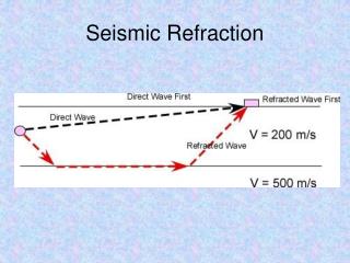
RAYINVR (Zelt and Smith, 1992; Zelt, 1999) • Model parameterization: • 2D velocity model is composed of a sequence of layers; Each layer boundary is defined by boundary nodes connected by straight-line segments of arbitrary dip; Vertical boundaries separate each layer into trapezoidal blocks; Velocity varies linearly between velocity points located on layer boundaries; Velocity discontinuities resulting in reflections are defined by upper and lower layer velocity points at selected boundary nodes • Forward problem: • Traveltimes through velocity model computed using zero-order asymptotic ray theory by solving the ray tracing equations numerically • Inverse problem: • Damped least-squares inversion; Can be limited to a set of model parameters • Goal: • Develop a detailed velocity model of the subsurface by applying a top-down layer-stripping approach; Fit various seismic phases to first constrain shallow structure and then progressively construct the deeper layers

Strategies for modelling seismic refraction/wide-angle reflection travel-times to obtain 2-D velocity and interface structure Given the unique characteristics of each data set and the local earth structure, there is no single approach to modelling wide-angle data that is best. The Zelt (1999) paper describes the best modelling strategies according to (1) the model parametrization, (2) the inclusion of prior information, (3) the complexity of the earth structure, (4) the characteristics of the data, and (5) the utilization of coincident seismic reflection data. The most important advantages of an inverse method are the ability to derive simpler models for the appropriate level of fit to the data, and the ability to assess the final model in terms of resolution, parameter bounds and non-uniqueness. [However,] if there is strong lateral heterogeneity in the near-surface only, layer stripping works well. Direct model assessment techniques that derive alternative models that satisfactorily fit the real data are the best means of establishing the absolute bounds on model parameters and whether a particular model feature is required by the data.

With good-quality reflection data, the final section can often be presented in un-interpreted form so that the reader can assess the interpretation provided and objectively establish their own interpretation. With wide-angle data, the primary goal is to produce a velocity model that predicts the observed travel-times. Thus, the final result of the modelling approach, the model, is fundamentally different from the result of the processing approach, since it looks nothing like the data. It is left to the modeller to establish the credibility of the model, usually through ray diagrams, overlaying the data with predicted times, comparing the observed and predicted times directly, or presenting the diagonal values of the resolution matrix. These methods are insufficient because of the non-uniqueness of the problem; that is, none of these displays address whether particular model structure is required by the data and what range of models fit the data.

A model developed by the analysis of wide-angle travel-time is only as good as the picks. Arrivals should only be included in the modelling once they can be confidently identified. Assigning layers to refracted arrivals may unnecessarily bias the modelling process. In obvious cases it may be worthwhile to identify the refracting layer since it may help to stabilize an inversion or supply more confidence when forward modelling. The use of fully automated picking routines is uncommon, particularly for later arrivals. An efficient approach is a semi-automated scheme whereby a few picks are made interactively, and the intervening picks are determined automatically using a cross-correlation scheme. Picks should not be interpolated to provide a uniform spatial coverage, especially when there are significant data gaps, since this will provide an incorrect sense of model resolution. Assigning uncertainties to the arrival picks is necessary, to avoid over- or under- fitting the data. Datafitting is strongly linked with the data uncertainties. Ideally, an overall normalized χ2 travel-time misfit of 1 should be achieved [NB: but may require dense node spacings that result in poor resolution].

Refraction/reflection traveltime modeling/inversion using RAYINVR

Refraction/reflection traveltime modeling/inversion using RAYINVR NB: For marine case, s=receiver is fixed along line and r=shot position varies to give correct ranges for each receiver. Best fit line = great circle path. Flat earth valid for ranges < 500 km.

Refraction/reflection traveltime modeling/inversion using RAYINVR Starting Model

Inversion Strategies uniform/fine grid minimumstructure tomography Full inversion Model testing non-uniform/ coarse grid non-minimum (prior) structure Partial (top-down/ layer stripping) inversion Ray Invr Node spacing ≈ receiver spacing (0.5 near surface)

Refraction/reflection traveltime modeling/inversion using RAYINVR Cratonic continent oceanic margin

Some Examples from Dalhousie

Refraction/reflection traveltime modeling/inversion using RAYINVR Gerlings et al., 2011

Refraction/reflection traveltime modeling/inversion using RAYINVR Lau et al., 2006

Refraction/reflection traveltime modeling/inversion using RAYINVR Funck et al., 2004

Refraction/reflection traveltime modeling/inversion using RAYINVR Lau et al., 2006

Refraction/reflection traveltime modeling/inversion using RAYINVR OBS OBS 14 Lau et al., 2006

Refraction/reflection traveltime modeling/inversion using RAYINVR Wu et al., 2006

Refraction/reflection traveltime modeling/inversion using RAYINVR • Summary for RAYINVR Modeling • Forces model into a limited number of discrete layers which may or may not correspond to geological boundaries – e.g. changes in velocity gradient require separate layers not necessarily related to structure. • Modeler needs to define arrivals by layer number and type of arrival (i.e. reflection or refraction). Proceed with forward models from top to bottom using as few layers as possible. • Inversion rarely works for entire model unless highly simplified – e.g. for continental crust with simple boundaries and only a few layers. Generally need to limit inversion to one layer at a time. • Uncertainties in crustal velocities and boundaries are typically ± 0.1 km/s and ± 1-2 km with good control and ± 0.2-0.3 km/s and ± 5 km for poorer control. • For marine data, works best with coincident reflection data to define upper layer geometry (i.e. sediment and basement) and compare deeper structure between reflections and velocity model.

References Funck, T., Jackson, H.R., Louden, K.E., Dehler, S.A.& Wu,Y., 2004. Crustal structure of the northern Nova Scotia rifted continental margin (Eastern Canada), J. geophys. Res., 109, B09102, doi:10.1019/2004JB003008. Gerlings, J., Louden, K.E., & Jackson, J.R., 2011, Crustal structure of the Flemish Cap Continental Margin (Eastern Canada): An analysis of a seismic refraction profile, Geophys. J. Int., 185, 30-48. Lau K.W.H., Louden, K.E., Funck, T., Tucholke, B.E., Holbrook, W.S., Hopper, J.R. & Larsen, H.C., 2006. Crustal structure across the Grand Banks–Newfoundland Basin Continental Margin–I. Results from a seismic refraction profile, Geophys. J. Int., 167, 127–156. Wu, Y., Louden, K.E., Funck, T., Jackson, H.R., & Dehler, S.A., 2006. Crustal structure of the central Nova Scotia margin off Eastern Canada, Geophy. J. Int., 166, 878–906. Zelt, C.A., 1999. Modeling strategies and model assessment for wide-angle seismic traveltime data, Geophys. J. Int., 139, 183–204. Zelt, A.C.& Smith, R.B., 1992. Seismic travel time inversion for 2-D crustal velocity structure, Geophys. J. Int., 108, 16–34.

Seismic Refraction Layer Modelling in 2D