Seismic Refraction
Seismic Refraction. Let’s start off with the simple ray of energy at a boundary …. Incident wave. Layer 1. Layer 2 velocity > Layer 1 velocity. Layer 2. Some energy is reflected …. r = i. Incident wave. Reflected wave. Layer 1. Layer 2 velocity > Layer 1 velocity. Layer 2.

Seismic Refraction
E N D
Presentation Transcript
Let’s start off with the simple ray of energy at a boundary … Incident wave Layer 1 Layer 2 velocity > Layer 1 velocity Layer 2
Some energy is reflected … r = i Incident wave Reflected wave Layer 1 Layer 2 velocity > Layer 1 velocity Layer 2 at an angle equal to the angle of incidence.
r = i Incident wave Reflected wave Layer 1 Layer 2 velocity > Layer 1 velocity Layer 2 This follows from Snell’s Law, that for a velocity V: V/sinf = constant, where f is the angle.
This is the basis for seismic and radar reflection. r = i Incident wave Reflected wave Layer 1 Layer 2 velocity > Layer 1 velocity Layer 2
We can also get some energy transmitted or refracted … Incident wave Reflected wave Layer 1 Layer 2 velocity > Layer 1 velocity Layer 2 > Refracted wave at an angle R, which also satisfies Snell’s Law.
From Snell’s law, V1/sini = V2/sinR Incident wave Reflected wave Layer 1 Layer 2 velocity > Layer 1 velocity Layer 2 > Refracted wave which tells us that R = sin-1 (V2sini/V1)
As the angle of incidence, i, increases, so too do r and R. Incident wave Reflected wave Layer 1 Layer 2 velocity > Layer 1 velocity Layer 2 > Refracted wave
As the angle of incidence, i, increases, so too do r and R. Incident wave Reflected wave Layer 1 Layer 2 velocity > Layer 1 velocity Layer 2 > Refracted wave
At some point, the angle of incidence becomes large enough … Incident wave Reflected wave Layer 1 Refracted wave Layer 2 velocity > Layer 1 velocity Layer 2 > that the angle of refraction equals90°, and the refracted ray follows along the boundary.
This occurs when V1/sini = V2/sin 90° = V2, or sini = V1/V2. Incident wave Reflected wave Layer 1 Refracted wave Layer 2 velocity > Layer 1 velocity Layer 2 >
As the refracted wave travels along the boundary … Incident wave Head waves Reflected wave Layer 1 Refracted wave Layer 2 velocity > Layer 1 velocity Layer 2 > it interacts with the boundary and sends energy back to the surface in the form of what are called “head waves”.
Layer 1 (low velocity) Layer 2 (high velocity) Time (sec or ms) Distance S R h
Layer 1 (low velocity) Layer 2 (high velocity) Time (sec or ms) Dx Dt Slope = Dt/Dx = 1/V1 Xcrit Distance First refractions S R h
Layer 1 (low velocity) Layer 2 (high velocity) Time (sec or ms) Xcrit Distance First refractions S R h
Layer 1 (low velocity) Layer 2 (high velocity) Time (sec or ms) Xcrit Xcros Distance First refractions S R h
Layer 1 (low velocity) Layer 2 (high velocity) Time (sec or ms) Xcrit Xcros Distance First refractions S R h
Layer 2 (high velocity) Dt Dx Slope = Dt/Dx = 1/V2 Time (sec or ms) Xcrit Xcros Distance First refractions S R h
That can be extended to however many layers. BUT … not always. There are some problems with refraction. These are called “hidden layer” problems, and there are two main types:
Layer 3 Time Layer 2 Layer 1 (a-ii) Distance
Layer 2 Layer 3 Time Layer 1 (a-iii) Distance Thin layer
Layer 3 Time Layer 1 (b) Distance Low velocity layer
V = 300 m/ms • 100 – 150 m/ms • 60 – 80 m/ms Water table Low velocity layer This is where radar refraction comes in … So radar refraction in general is not viable. Returning to seismic refraction … what about dipping and undulating layers and surfaces?
S 2 S 2 S 1 S 1
Updip S2 Downdip S 1 S1 S2
First we send a shot one way along a traverse … S R It takes a certain amount of time, tF A-B from A to B. (from beginning to end)
First we send a shot one way along a traverse … S R It takes a certain amount of travel time, tF, from A to R.
Then we send a shot the other way along a traverse … S S R It takes a certain amount of time, tR B-A from B to A. (from beginning to end)
Then we send a shot the other way along a traverse … S S R It takes a certain amount of travel time, tR, from B to R.
We combine the results for both shots … S S R The total time between A and B is the average of the forward and reverse times, called the reciprocal time: TR = (tF A-B + tR B-A)/2.
We combine the results for both shots … S S R The average refraction time from A to R and from B to R is the average of the forward and reverse times: (tF + tR)/2.
Time depth We combine the results for both shots … S S R The residual time, called the time depth, is the average extra time taken for the refracted energy to travel to R rather than bypass that “detour”.
Time depth We combine the results for both shots … S S R That extra time, the time depth, is equal to the average refraction time with the total time removed: td = (tF + tR – TR)/2
Time depth The shaded triangle shows the area of influence. S S R The forward and reverse refractions are governed by the V contrast, V1/V2, at that specific segment of the boundary and the time delay is related to the depth atthatpoint.
Time depth S S R The forward and reverse refraction times are corrected by removing the time delay, td, and what’s left is only the velocity contrast, V1/V2, at that segment of the boundary: tF corr = tF – td and tR corr = tR – td .
Time depth When we plot tF corr and tR corr vs distance … S S R we get straight lines that represent V2 at each boundary segment.
Time depth This technique was developed by Derecke Palmer (1983). S S R It is called the Generalised Reciprocal Method (GRM), and can be generalised to any number of layers.
Time depth This technique was developed by Derecke Palmer (1983). Usable arrivals for GRM analysis S S R It is called the Generalised Reciprocal Method (GRM), and can be generalised to any number of layers. BUT … it can only be applied when there are refractions from BOTH directions. Direct arrivals cannot be used.
We can also do ray-tracing and fan shooting, which ultimately are versions of tomographic reconstruction.
Some rays miss the “target” (the anomalous feature) and have no time anomaly (slower or faster).
Conversely some rays catch the “target” to different degrees, and thus have anomalous travel times.
We shoot from different angles and perspectives and thus can build up a picture of the anomalous feature.