WinSism refraction seismic of W_GeoSoft Geo2 X SA
WinSism refraction seismic of W_GeoSoft Geo2 X SA. How to use the software ?. Compatibiliy. Window 7,8 (PDF display problem) Window Xp (no known problem) Windows 95, 98 (no known problem) Windows 2000 & NT (Occasional compatibility problems) Windows Me (Few feedback…).

WinSism refraction seismic of W_GeoSoft Geo2 X SA
E N D
Presentation Transcript
WinSism refraction seismicof W_GeoSoftGeo2XSA How to use the software ?
Compatibiliy • Window 7,8 (PDF display problem) • Window Xp (no known problem) • Windows 95, 98 (no known problem) • Windows 2000 & NT (Occasional compatibility problems) • Windows Me (Few feedback…)
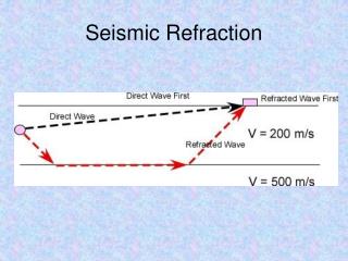
Few abbreviations to know • TT= travel time • FBP= First break point • IT=Intercept times • BR=Bedrock • GRM= Generalized Reciprocal Method • SU=Seismic Unix
First you must convert your field data to SU format Click here Then select your file format
To convert SEG2 to SU, just select all records of a spread Select your records Convert to Su format All shots data of one spread will be recorded into one large SU file !!!, Shot order must be the same as field recording order, shot 1 = first offset, shot 2=end shot 1
First break picking is the next stepPrecise picking is fundamental! Select the SU file Use the scroll bar to select record Pick the FBP (First break points) You can enlarge trace size, clip amplitudes and more… With the mouse reduce time display
How tu use automatic picking First, click on the smallest break time with the right button The move the scroll to adjust all FBP automatically If necessary adjust parameters Picking can be corrected later
Travel time structure • To give valuable informations a seismic refraction spread MUST have at least 2 offsets, 2 end shots one center shot (see REDPATH booklet) ! • You can have up to 48 shots and 96 receivers per shot • Distance ZERO is END SHOT 1 • Offset 1 will have a negative distance • All receiver distances are measured from END SHOT 1
Now, we can build the travel time (1) • You must enter few data • File name • Geophone spacing and number • Shot spacing and number
Build the travel time (2) Double click on the top first cell of shot 1 and the select the corresponding FBP file. Repeat for all shots Time delay can be added to all times FBP files can be renamed when used or reversed
Build the travel time (3) Click on SAVE and DISPLAY Repeat for all shot and correct if necessary shot location and elevation
Build the travel time (4) Display and control the travel time Zoom is possible
Travel time correction 1 Select and display the SU file Click on the FPB to correct Travel time is updated automatically If necessary adjust display parameters
Travel time correction 2 Correct the value on the grid then click on SAVE and DISPLAY button
Travel time correction 3 You can move any FBP time, double click on a point, keep pressed and release the mouse at the new correct location. To delete a point, double click on it and release without moving.
Bed rock velocity determination To know the BR velocity use the true velocity between the two offset shots If you have not a straight line, you can have more than one BR velocity If you know the number of layers save the BR velocity
Travel time moving You can move the offset shot down to the End shot Bedrock arrivals • You can determine: • Which part of the End shot belongs to bedrock • The intercept time for the end shot (Save it) First and second layer arrivals
Velocity determination (1): Linear regression Select a shot first and last geophone Compute using linear regression and save the velocity for the correct layer number
Velocity determination (2) You can draw a line with the mouse (Down, move Up), velocity is computed and can be saved (Menu PROCESSINGVELOCITY DETERMINATION)
Depth computation Intercept Time method When all layer velocities and IT have been determined, you can compute the layer thicknesses and BR depth Select shot Compute Save if not automatic
Coloured profile display (1) Select the PROFILE PARAMETER tab And enter your choices Profile elevation and thickness Draw shot or/and geophones Click here to prepare the profile
Coloured profile display (2) This graph can be saved as WMF, JPG file or copy into the clipboard and PASTE into any program (WORD, PAINT, CORELDRAW) Click on right button to launch graph editor
ABC method (1) Move down the offset travel time to fit as well as possible on the end shots
ABC method (2) Move the total time line down to the end of shots You can now compute time from surface to bedrock below all geophones Delay times give a good idea of bedrock geometry, like furrows
ABC method (3) If you already compute depth below shots, you can know the bedrock depth below all receivers
ABC method (4) You can also display a ABC coloured profile
GRM method (1) This method is not suitable if you have less than 24 geophones First have a look on the velocity fonction curve to select the receiver spacing See the PALMER thesis PDF file in theW_GeoSoftCD-ROM for all theory
GRM method (2) Then the Time depth curve is drawn
GRM method (3) Last step, depth computation below all geophones and save the values in the GRM grid file
GRM method (4) Using the GRM file, you can draw a coloured profile of GRM depth computation
Quick interpretation You can have easily a first idea of depth with the QUICK INTERPRETATION module. The Just select the shot number, the number of layer and move the layer limit You can save depth and velocities in the WinSism WS4 file
WinSism menu Most of the operations can be launched using pictograms or shortcuts Thickness computation Printing Display profile ABC method GRM Method Zoom FB picking Redisplay TT File info Correct a TT Build TT Quick interpretation Trace moving Velocity linear regression Velocity point to point Velocity line True velocity Help Ruler EXIT Display a TT Read a WinSism file Save a WinSism file Convert field records