Download
1 / 31
560 likes | 1.87k Vues
Coherent MIMO Radar: High Resolution Applications. Alex Haimovich New Jersey Institute of Technology Princeton, Nov. 15 2007. Overview. Radar Problem What is MIMO radar Signal model Non-coherent mode Coherent mode GDOP Summary. Radar Problem.

E N D
Coherent MIMO Radar:High Resolution Applications Alex Haimovich New Jersey Institute of Technology Princeton, Nov. 15 2007
Overview • Radar Problem • What is MIMO radar • Signal model • Non-coherent mode • Coherent mode • GDOP • Summary
Radar Problem • In its simplest form, the radar problem is: given a transmitted a waveform s(t) known to the receiver, and observing a returned signal r(t) r(t) = s(t-τ) + noise, - detect the presence of a target - estimate the target range r0 from its relation to the time delay τ = 2r0/c • If target has range rate (velocity) v0, then r(t) will acquire a Doppler shift fd = (2v0/c)f0 - estimate the range rate from the frequency shift r(t) = s(t-τ)ej2πfd(t-τ) + noise • Estimate target angle utilizing a directional antenna or an antenna array
Radar Measurements Detection • A complex target, such as an airplane, comprises many independent scatterers • The target echo has envelope with a Rayleigh distribution • Target fading affects received SNR; lower probability of target detection Range estimation • Range resolution scales with 1/(signal bandwidth) Range rate estimation • Uncertainty principle in radar: it is not possible to measure both range and range rate with arbitrary resolution • Angle measurement resolution ~ λ/L, λ is carrier wavelength, L is antenna aperture size
Conventional Techniques • Target localization in a resolution cell range resolution = 1/(signal bandwidth) cross range resolution = beamwidth x range to target • Improve detection: transmit higher power; spread spectrum gain • Improve range resolution: transmit higher bandwidth waveform • Improve cross-range resolution: use larger aperture antenna • An antenna array has an aperture that scales with the number of sensors
MIMO-radar Tx Rx What is MIMO Radar? MIMO radar: a radar system that employs multiple transmit waveforms and has the ability to jointly process signals received at multiple antennas • Independent waveforms: omnidirectional beampattern • Diverse beampatterns created by controlling correlations among transmitted waveforms Antenna elements of MIMO radar can be co-located or distributed
MIMO-radar Phased array radar Multistatic radar Tx Tx SP SP SP SP Rx Tx Rx Related Radar Architectures • MIMO radar: diversity of waveforms; centralized processing for target detection, localization • Multistatic: typically, single illuminator and receivers that act as independent radars • Phased array: single waveform and centralized processing of received signals
Why MIMO Radar? • Co-located sensors • Omnidirectional space illumination • Reduced coherent energy on target • All the benefits of coherent beams obtained post-processing • Distributed sensors • Extended target acts as channel with spatial selectivity – target radar cross section (RCS) diversity • High resolution localization • Multiplicity of sensors supports high accuracy localization • Handling of multiple targets • Improved Doppler processing through diversity of look angles and mitigation of the problem of low radial velocities Backscatter as a function of azimuth angle, 10-cm wavelength [Skolnik 2003].
MIMO Radar Channel Assumptions: • Target consists of point scatterers distributed within the target’s volume • Scatterers have complex-value, i.i.d. response • All tx-target-rx paths have the same pathloss • Near field signal model: sensors-scatterers paths have own angle, range Path gains from transmit antenna k to receive antenna ℓ, hℓk are organized in a matrix H = [hℓk]. H can be expressed: H = KΕG: • K: phase shifts due to paths transmitters to scatterers • Ε scatterers response • G phase shifts due to paths scatterers to receivers
Earlier Results Results (Fishler et. al. 2004): • For a sufficiently large number of scatterers, the channel elements hℓk are complex-value, jointly Gaussian • For sufficiently separated antenna elements, the channel elements hℓk are iid, i.e., the channel matrix H is likely to have full rank The elements of the matrix H are unknown, their statistics are known
Rx Tx Rx1 M N Rx2 Tx1 Tx2 Comm vs. Radar Channels • Sufficient conditions for full-rank H: • Each scatterer receives signals uncorrelated to any other scatterer: different scatterers fall in different transmit array beams • Each receive antenna observes signals uncorrelated to any other antenna: different receive antennas fall in different beamwidths of the scatterers • MIMO comm.: antennas are co-located; scatterers are separated • MIMO radar: antennas are separated; scatterers are co-located MIMO comm channel MIMO radar channel
Comm vs. Radar Signal Models • MIMO comm • Detection of space-time coded digital symbols (e.g., PSK, QAM) sk(t) • Channel coefficients hℓk known/estimated (coherent communication) • MIMO radar • Transmitted waveforms sk(t)are known to the receiver • Channel coefficients are unknown • Target localization is essentially a delay estimation problem: • Non-coherent: measurement of signal envelopes • Coherent: measurements of signal envelopes and phases MIMO Comm MIMO Radar
Radar 2 Radar 3 Radar 1 Radar 4 Radar 5 Non-coherent MIMO Radar • Processing based only on time delay measurements • Resolution cell (c/B) x (c/B), B bandwidth of transmitted waveform • Since “channel” is not known, orthogonal waveforms are needed to separate signals at the receiver • Exploit non-coherent diversity paths
Non-coherent Localization Applications: • Multiple targets at long distance. Each target appears as point scatterer. • Targets are unresolvable by radar waveform • This model results in RCS diversity, i.e., full rank channel matrix H • Channel matrix H is unknown, its pdf is known RCS center of gravity c/B Distinguishing features of non-coherent MIMO radar: • Orthogonal waveforms • Time delay measurements only (non-coherent) MIMO “gain” • Illumination of full surveillance volume • Exploit RCS diversity • Geometric dilution of precision (GDOP) advantage of the radar system footprint
Spatial Diversity Gain in Radar Miss probability of MIMO radar compared to conventional phased-array. Miss probability is plotted versus SNR for a fixed false alarm probability of 10-6.
Coherent Mode • Non-coherent mode identified a target of interest • Now, switch to high resolution, coherent mode to investigate the target • Goal is to obtain resolution beyond possible with the radar waveform • Refined location estimation carried out in the neighborhood of the nominal target location X0 = (x0,y0). • Requires phase synchronization of distributed sensors Rx (xrl,yrl) Tx (xtk,ytk) yc+ y (x0,y0) rl tk (xc,yc) xc+x Nominal target location MIMO radar signal model.
Beamforming Modes • Various modes of operation are possible with M transmit x N receive antennas, and coherent processing • The channel matrix H is estimated at the nominal target location X0 • Under some conditions, the rank of H indicates the number of targets in the field of view of the MIMO radar Beamforming mode • Signals at transmit antennas are co-phased to generate a beam • Up to M orthogonal beams can be generated simultaneously Grid of beams
MIMO Modes • Similarly, 1 to N beams can be generated at the receiver • Each resolution cell: wavelength x range to target / array baseline MIMO mode • Transmit antennas emit independent waveforms • Uniform spatial illumination – low coherent energy on targets • Receiver processing: • Scan resolution cells with single/grid of beams MIMO
Coherent Signal Model • Signal measured by lth radar for point target located at X: E/M is the signal energy, wl(t) is a white Gaussian noise, ς target complex gain, and lk(X0) is a phase factor dependent on the target location relative sensors k and l. • Likelihood L(r;),function of observations and unknown parameters: Vector of unknown parameters = [x, y, ]T.
Resolution • Setup: • Sensor locations (M=N=9): • [-40, -35, -15, -2, 5, 10, 18, 25, 40] • Sensor locations (M=N=2): [20, 40] • Bandwidth to carrier frequency ratio = 1/1000 • Target location [0, 0] • All radars assumed to be in transmit/receive mode
Localization Error • Different ways to estimate target location, and evaluate the performance of the estimate: • ML estimate of = [x, y, ]T; target reflectivity is nuisance parameter • Best linear unbiased estimate (BLUE) – exploit linear model for time delay • The error covariance matrix is lower bounded by the Cramér-Rao Lower Bound (CRLB): • The CRLB is given by the inverse of the Fisher Information Matrix (FIM) IF():
Linear Perturbation Model • The time delay of the signal sk(t) transmitted by radar k, located at (xtk,ytk) , reflected by a target located at X = (x,y) and received by radar l located at (xrl,yrl) : c = 3x10⁸ m/s is the speed of light. • Time delay is nonlinear function of target location • Linear perturbation model: linearize around nominal location (xc,yc) Rx (xrl,yrl) Tx (xtk,ytk) yc+ y (x0,y0) rl • tk, rl: azimuth angles • Multiple, point targets; homogeneous, unknown complex gains = r+ j i tk (xc,yc) xc+x Nominal target location
BLUE Localization • Postulate linear model between time delays and unknown target location • Linear observations model: time delays are the observables (θ) = Dθ+ D is the observation matrix containing angle terms (θ) = [11, 12, 13,…, MN]T are time delays = [11, 12,…, MN]T are time delay measurement errors, assumed iid Gaussian, zero-mean, covariance C θ=[x, y, ]T, where defines a range measurement error • How is BLUE performed?
BLUE Localization Target localization : • ML estimate of time delays τℓk • The estimated time delays serve as “observations” of the signal model (θ) = Dθ+ • Time delay estimation errors serve as the measurement errors kℓ • Relation between time delay and target location: • The locus of constant sum of time delays “transmitter k – target” and “target – receiver ℓ” is an ellipse • The target location is found at the intersection of ellipses formed with pairs of transmitter-receiver as foci • BLUE target localization, and BLUE covariance matrix of the estimate
BLUE Features • For the BLUE, the estimation error covariance matrix is: • The term uB and the matrix GB incorporate the effect of sensor locations relative to the target • The term β is the effective bandwidth • We are interested in the variances σx2, σy2 of the estimates of the x and y coordinates of the target (terms 1,1 and 2,2 in CBLUE) • For the linear, Gaussian model, BLUE is asymptotically (long observation time) optimal, i.e., meets CRLB • Localization error is approximately proportional to 1/ fc2 • The effective bandwidth β has little impact • What is the relation between sensor locations and localization error?
Geometric Dilution of Precision • Geometric Dilution Of Precision (GDOP) metric is commonly used in global positioning systems (GPS) in mapping the attainable location accuracy for a given layout of GPS satellites • GDOP enables to separate the effect of geometry from the effect of measurement error • Given a linear measurement model of the time delays with noise variance (same model as used for BLUE), the GDOP is given by • Since the BLUE and its covariance matrix are given in closed-form, the GDOP can be also calculated in closed-form
Lowest GDOP • The lowest GDOP corresponds to the most favorable geometry for the problem • At least 3 sensors are required to resolve location ambiguity • Assumptions for calculating GDOP: • A regular N-sided polygon is centered at the axis origin (x = 0, y = 0) and the target is located at its center. • M = N radars transmitting/receiving radars located at the polygon vertices • GDOP for BLUE localization is: • It can be shown that this is the lowest attainable GDOP
GDOP Numerical Examples • Example 1: Three and five radars, located symmetrically around the axis origin. All are both transmit and receive radars, i.e., N=M=3 and N=M=5 for the first and second case, respectively. GDOP contours for M = N = 3 GDOP contours for M = N = 5
Discussion Features • Earlier we listed features of non-coherent MIMO radar. Contrast those with coherent MIMO radar. • Orthogonal waveforms • Orthogonal waveforms enable to illuminate the whole surveillance space • Estimate the number of targets/scatterers through the rank of the channel matrix H • Time delay measurements only (non-coherent) • Time delay estimation by way of phase measurements MIMO “gain” • Illumination of full surveillance volume • Ability to estimate multiple targets through multiple receive beams • High resolution, but with ambiguities; ambiguities are reduced through increasing the number of sensors • High accuracy target localization: scales with 1/(SNR x fc2) • GDOP advantage sqrt(2)/M
Concluding Remarks • Under some conditions, the MIMO radar signal model has similarities to the MIMO communications signal model. In particular, it includes a channel matrix with uncorrelated elements. • Non-coherent MIMO radar seeks to exploit target RCS diversity to improve detection and estimation performance. • Coherent MIMO radar supports high resolution, albeit ambiguous target localization. • Ambiguities can be controlled through the number of sensors. • Localization with coherent MIMO radar exhibits an error that scales with 1/carrier frequency2 • The GDOP was introduced for the analysis of the more complex terms of the covariance matrix and the CRLB. This graphical representation provides comprehensive tool for the evaluation of the radar locations effect on the attainable accuracy at a given region. • The use of multiple sensors improves localization accuracy by a factor as low as sqrt(2)/M, where M is the number of transmit and receive antennas.
Open Questions • MIMO radar signal optimization for range and range rate estimation • Signals with low cross correlations over a range of delays • Signal design for reducing localization ambiguities • Study the statistics of ambiguities and relations to the various parameters: carrier frequency, bandwidth, number of sensors • Characterizing the performance of MIMO radar at low SNR (in the presence of noise ambiguities) • Handling multiple targets