Download
1 / 21
220 likes | 492 Vues
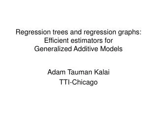
Regression trees and regression graphs: Efficient estimators for Generalized Additive Models . Adam Tauman Kalai TTI-Chicago. Outline. Generalized Additive Models (GAM) Computationally efficient regression Model Thm: Regression graph algorithm efficiently learns GAMs

E N D
Regression trees and regression graphs:Efficient estimators for Generalized Additive Models Adam Tauman Kalai TTI-Chicago
Outline • Generalized Additive Models (GAM) • Computationally efficient regression • Model Thm: Regression graph algorithm efficiently learns GAMs • Regression tree algorithm • Regression graph algorithm Correlation boosting • [Valiant] [Kearns&Schapire] New [Mansour&McAllester] New
Generalized Additive Models[Hastie & Tibshirani] • e.g., Generalized linear models • u( w¢x ), monotonic u • linear/logistic models • e.g., f(x) = e–||x||2 = e–x(1)2–x(2)2…–x(d)2 Dist. over X£Y = Rd£R f(x) = E[y|x] = u(f1(x(1))+f2(x(2))+…+fd(x(d))) monotonic u: R!R, arbitrary fi: R!R
Non-Hodgkin’s Lymphoma International Prognostics Index [NEJM ‘93] Risk Factors age>60, # sites>1, perf. status>1, LDH>normal, stage>2
Setup X £Y .1 1 1 1 0 .4 .4 0 1 0 0 .3 0 0 1 1 1 0 0 1 .1 1 1 1 0 0 .2 1 1 0 1 regression algorithm 0 1 1 0 .3 1 1 1 1 0 0 1 .8 0 1 .3 0 1 1 1 .4 1 .4 0 1 1 1 0 .5 0 1 1 .7 1 1 0 0 0 0 1 0 0 0 1 0 1 1 1 0 1 0 0 .3 1 1 1 1 1 1 0 1 1 “training error” (h,train) = i(h(xi)-y)2 0 0 0 0 0 .2 0 0 1 0 0 0 .02 1 0 0 1 1 .5 0 0 0 0 1 1 .4 0 0 0 0 1 .2 0 0 0 1 0 1 0 0 1 1 .2 0 1 0 1 .3 1 n 0 0 h: X! [0,1] “true error” (h) = E[(h(x)-y)2] X = RdY = [0,1] training sample: (x1,y1),…,(xn,yn)
X £ [0,1] h: X! [0,1] Computationally-efficient regression [Kearns&Schapire] Family of target functions Definition: A efficiently learns F: f(x) = E[y|x] 2F, 8 with probability 1-, >0 E[(h(x)-y)2] · E[(f(x)-y)2]+(term)/nc n examples true error (h) poly(|f|,1/) Learning Algorithm A A’s runtime must be poly(n,|f|)
Outline • Generalized Additive Models (GAM) • Computationally efficient regression • Model Thm: Regression graph algorithm efficiently learns GAMs • Regression tree algorithm • Regression graph algorithm Correlation boosting • [Valiant] [Kearns&Schapire] New [Mansour&McAllester] New
New Results for GAM’s 1 .1 1 0 0 .6 0 0 0 .7 0 1 1 Regression Graph Learner 0 0 .8 1 .4 0 1 .2 1 1 1 1 0 1 1 0 1 h: Rd ![0,1] n samples 2 X £ [0,1] X µRd Thm:reg. graph learner efficiently learns GAMs • 8dist over X£Y with E[y|x] = f(x) 2 GAM • E[(h(x)-y)2] · E[(f(x)-y)2] + O(LV log(dn/)) • runtime = poly(n,d) 8 with probability 1-, n1/7
New Results for GAM’s • f(x) = u(i fi(x(i))) • u: R!R, monotonic, L-Lipschitz (L=max |u’(z)|) • fi: R!R, bounded total variationV = i s |fi’(z)|dz Thm:reg. graph learner efficiently learns GAMs • 8dist over X£Y with E[y|x]=f(x) 2 GAM • E[(h(x)-y)2] · E[(f(x)-y)2] + O(LV log(dn/)) • runtime = poly(n,d) n1/7
New Results for GAM’s 1 .1 0 0 .6 0 0 1 0 .7 0 1 1 Regression Tree Learner 0 0 .8 1 .4 0 1 .2 1 1 1 1 0 1 1 0 1 h: Rd ![0,1] n samples 2 X £ [0,1] X µRd Thm:reg. tree learner inefficiently learns GAMs • 8dist over X£Y with E[y|x]=f(x) 2 GAM • E[(h(x)-y)2] · E[(f(x)-y)2] + O(LV) • runtime = poly(n,d) ( ) 1/4 log(d) log(n)
Regression Tree Algorithm • Regression tree RT: Rd! [0,1] • Training sample (x1,y1),(x2,y2),…,(xn,yn) 2Rd£ [0,1] (x1,y1), (x2,y2), … avg(y1,y2,…,yn)
Regression Tree Algorithm • Regression tree RT: Rd! [0,1] • Training sample (x1,y1),(x2,y2),…,(xn,yn) 2Rd£ [0,1] x(j) ¸ ? (xi,yi): x(j) < (xi,yi): x(j) ¸ avg(yi: xi(j)<) avg(yi: xi(j)¸)
Regression Tree Algorithm • Regression tree RT: Rd! [0,1] • Training sample (x1,y1),(x2,y2),…,(xn,yn) 2Rd£ [0,1] x(j) ¸ ? (xi,yi): x(j) < x(j’) ¸’ ? avg(yi: xi(j)<) (xi,yi): x(j) ¸ andx(j’)< ’ (xi,yi): x(j) ¸ andx(j’) ¸’ avg(yi: x(j)¸Æx(j’)¸’) avg(yi: x(j)¸Æx(j’)<’)
Regression Tree Algorithm • n = amount of training data • Put all data into one leaf • Repeat until size(RT)=n/log2(n): • Greedily choose leaf and split x(j) · to minimize (RT,train) = (RT(xi)-yi)2/n • Divide data in split node into two new leaves Equivalent to “Gini”
Regression Graph Algorithm [Mansour&McAllester] • Regression graph RG: Rd! [0,1] • Training sample (x1,y1),(x2,y2),…,(xn,yn) 2Rd£ [0,1] x(j) ¸ ? x(j’’) ¸’’ ? x(j’) ¸’ ? (xi,yi): x(j) < andx(j’’)< ’’ (xi,yi): x(j) < andx(j’’) ¸’’ (xi,yi): x(j) ¸ andx(j’)< ’ (xi,yi): x(j) ¸ andx(j’) ¸’ avg(yi: x(j)¸Æx(j’)¸’) avg(yi: x(j)<Æx(j’’)<’’) avg(yi: x(j)¸Æx(j’)<’) avg(yi: x(j)<Æx(j’’)¸’’)
Regression Graph Algorithm [Mansour&McAllester] • Regression graph RG: Rd! [0,1] • Training sample (x1,y1),(x2,y2),…,(xn,yn) 2Rd£ [0,1] x(j) ¸ ? x(j’’) ¸’’ ? x(j’) ¸’ ? (xi,yi): x(j) < andx(j’’)< ’’ (xi,yi): x(j) < andx(j’’) ¸’’ or x(j) ¸ and x(j’) < ’ (xi,yi): x(j) ¸ andx(j’) ¸’ avg(yi: x(j)¸Æx(j’)¸’) avg(yi: x(j)<Æx(j’)<’) avg(yi: (x(j)<Æx(j’’)¸’’)Ç(x(j)¸Æx(j’)<’))
Regression Graph Algorithm [Mansour&McAllester] • Put all n training data into one leaf • Repeat until size(RG)=n3/7: • Split: greedily choose leaf and split x(j) · to minimize (RG,train) = (RG(xi)-yi)2/n • Divide data in split node into two new leaves • Let be the decrease in (RG,train) from this split • Merge(s): • Greedily choose two leaves whose merger increases (RG,train) as little as possible • Repeat merging while total increase in (RG,train) from merges is ·/2
Two useful lemmas • Uniform generalization bound for any n: • Existence of a correlated split:There always exists a split I(x(i) ·) s.t., regression graph R probability over training sets (x1,y1),…,(xn,yn)
Motivating natural example • X = {0,1}d, f(x) = (x(1)+x(2)+…+x(d))/d, uniform • Size(RT) ¼ exp(Size(RG)c), e.g. d=4: x(1)>½ x(1)>½ x(2)>½ x(2)>½ x(2)>½ x(2)>½ x(3)>½ x(3)>½ x(3)>½ x(4)>½ x(4)>½ x(4)>½ x(4)>½ x(3)>½ x(3)>½ x(3)>½ x(3)>½ 0 .25 .5 .75 1 x(4)>½ x(4)>½ x(4)>½ x(4)>½ x(4)>½ x(4)>½ x(4)>½ x(4)>½ .25 .5 .5 .75 .5 .75 .75 1 .25 .5 .5 .75 0 .25 .25 .5
Regression boosting • Incremental learning • Suppose you find something of positive correlation with y, then reg. graphs make progress • “Weak regression” implies strong regression, i.e. small correlations can efficiently be combined to get correlation near 1 (error near 0) • Generalizes binary classification boosting[Kearns&Valiant, Schapire, Mansour&McAllester,…]
Conclusions • Generalized additive models are very general • Regression graphs, i.e., regression trees with merging, provably estimate GAMs using polynomial data and runtime • Regression boosting generalizes binary classification boosting • Future work • Improve algorithm/analysis • Room for interesting work in statistics Å computational learning theory