Income and Expenditures Equilibrium
140 likes | 286 Vues
This document explores the concepts of income and expenditures equilibrium in economics, specifically focusing on the relationship between Aggregate Expenditure (AE) and Real GDP (Y). It discusses how changes in planned expenditure affect employment and output, highlighting the significance of the spending multiplier, which measures the effect of changes in autonomous expenditures on real GDP. Additionally, it examines factors such as the marginal propensity to save (MPS) and marginal propensity to import (MPI), and how they impact the multiplier effect, as well as addressing recessionary gaps and the path from aggregate expenditure to aggregate demand.

Income and Expenditures Equilibrium
E N D
Presentation Transcript
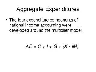
Movement to Equilibrium 45o line: AE = Y 700 Total Expenditure 600 Increase Output, increase Employment 500 Reduce Output, Reduce Employment Aggregate planned expenditure 400 0 300 400 500 600 700 Real GDP (Output)
Spending Multiplier • The spending multiplier measures the change in equilibrium income (real GDP) produced by change in autonomous expenditures: ΔY/ΔI = ΔY/ΔG = ΔY/ΔX • By how many dollars does real GDP change for every dollar change in autonomous expenditures?
Computing the Spending Multiplier:Marginal propensity to save = mps = .3Marginal propensity to import = mpi = .1 If MPS = 0.30 and MPI is 0.10, then MPS + MPI = 0.40 = 4/10. 1/0.40 = 1/(4/10) = 10/4 = 2.5 The multiplier is 2.5. NOTE: The spending multiplier would be larger in a closed economy because MPI would be zero.
GDP Gap, Recessionary Gap • GDP gap = potential real GDP – actual real GDP • How much does real GDP have to increase to generate full employment? • Recessionary gap • How much additional spending is needed to achieve potential GDP (to create full employment)?
