Download
1 / 32
320 likes | 439 Vues
Composite Analyses of Coupled Upper-Level Jet Streaks East of the Rocky Mountains. Chad M Gravelle Saint Louis University Scott M Rochette Thomas A Niziol

E N D
Composite Analyses of Coupled Upper-Level Jet Streaks East of the Rocky Mountains Chad M Gravelle Saint Louis University Scott M Rochette Thomas A Niziol State University of New York College at Brockport National Weather Service Forecast Office Buffalo Charles E Graves Saint Louis University Annual Missouri Academy of Science Meeting Missouri Western State University, 21 April 2007
Coupled Jet Streaks • The term ‘coupled jet streaks’ refers to the presence of two separate jet streaks juxtaposed in such fashion that the ascending branches of the transverse circulations are collocated with one another, resulting in an enhanced area of upward vertical motion (e.g., Uccellini and Kocin 1987). • This study will investigate coupled UL jet streak occurrences during the cool season Uccellini and Kocin 1987 (1 October to 31 March) east of the Rocky Mountains over 10 seasons (1993 – 2003).
Methodology • Preliminary examination using the North American Regional Reanalysis (NARR) dataset revealed 79 possible coupled jet streak occurrences during the period. • Using the General Meteorological Package (GEMPAK) with the NARR dataset, plan-view and cross-sectional analyses of the possible occurrences were analyzed to ensure the interaction of the jet streak circulations. • This revealed 39 coupled jet streak cases, which were then subdivided into weak dynamic (n=20) and strong dynamic (n=19) scenarios. • The weak dynamic cases were characterized by modest surface circulations (MSLP > 1000 hPa) and open mid-tropospheric waves. • The strong dynamic cases were characterized by strong surface circulations (MSLP < 1000 hPa) and closed mid-tropospheric waves.
Methodology • Center points between the jet streaks were then qualitatively determined by finding the midpoint on a line between the strongest common isotach for the initial coupling time, along with the prior 6- and 12-h time periods (see right). • A 117 x 117 grid with 32 km grid spacing was then extracted from the NARR dataset on the center points between the jet streaks. • The 20 cases were then averaged with a locally written compositing program utilizing the GEMPAK software.
Weak Dynamic Composites Locations of the center points for the 20 weak dynamic cases used in the composite analysis of the initial (t = 0h) coupling time.
Weak Dynamic Composites Composite analysis of 250-hPa isotachs (shaded, m s-1), 250-hPa heights (brown, gpdkm), 250-hPa ageostrophic wind vectors (red, m s-1), and 500-hPa omega (blue, -μbar s-1) at t = -12 h.
Weak Dynamic Composites Composite analysis of 250-hPa isotachs (shaded, m s-1), 250-hPa heights (brown, gpdkm), 250-hPa ageostrophic wind vectors (red, m s-1), and 500-hPa omega (blue, -μbar s-1) at t = 0 h.
Weak Dynamic Composites Composite analysis of 250-hPa isotachs (shaded, m s-1), 850-hPa isotachs (green, m s-1), and 850-hPa wind vectors (green, m s-1) at t = -12 h.
Weak Dynamic Composites Composite analysis of 250-hPa isotachs (shaded, m s-1), 850-hPa isotachs (green, m s-1), and 850-hPa wind vectors (green, m s-1) at t = 0 h.
Weak Dynamic Composites Composite analysis of 250-hPa isotachs (shaded, m s-1), 850-hPa wind vectors (green, m s-1), and 850-hPa theta-e advection (red, +K hr-1) at t = -12 h.
Weak Dynamic Composites Composite analysis of 250-hPa isotachs (shaded, m s-1), 850-hPa wind vectors (green, m s-1), and 850-hPa theta-e advection (red, +K hr-1) at t = 0 h.
Weak Dynamic Composites Composite analysis of 250-hPa isotachs (shaded, m s-1) and 850-hPa frontogenesis (red, +K [100 km]-1 [3 h] -1) at t = -12 h.
Weak Dynamic Composites Composite analysis of 250-hPa isotachs (shaded, m s-1) and 850-hPa frontogenesis (red, +K [100 km]-1 [3 h] -1) at t = 0 h.
Weak Dynamic Composites Composite analysis of 250-hPa isotachs (shaded, m s-1) and 1000-hPa heights (brown, gpm) at t = -12 h.
Weak Dynamic Composites Composite analysis of 250-hPa isotachs (shaded, m s-1) and 1000-hPa heights (brown, gpm) at t = 0 h.
Weak Dynamic Composites Composite cross section through the composite coupled jet streaks showing isotachs (green, m s-1), RH (>70%, green shading), ageostrophic circulation (blue arrows, m s-1), omega (red, -μbar s-1), and θe (black, K) at at t = -12 h. Inset figure provides the orientation of the cross-section with respect to the isotach field.
Weak Dynamic Composites Composite cross section through the composite coupled jet streaks showing isotachs (green, m s-1), RH (>70%, green shading), ageostrophic circulation (blue arrows, m s-1), omega (red, -μbar s-1), and θe (black, K) at at t = 0 h. Inset figure provides the orientation of the cross-section with respect to the isotach field.
Weak Dynamic Composites Composite cross section through the composite coupled jet streaks showing isotachs (green, m s-1), ageostrophic circulation (blue arrows, m s-1), frontogenesis (red, +10 K [100 km] -1 [3 h]-1), and EPVs (shaded, < 0.25 PVU) at t = -12 h.
Weak Dynamic Composites Composite cross section through the composite coupled jet streaks showing isotachs (green, m s-1), ageostrophic circulation (blue arrows, m s-1), frontogenesis (red, +10 K [100 km] -1 [3 h]-1), and EPVs (shaded, < 0.25 PVU) at t = 0 h.
Weak Dynamic Case Study • 8 March 2002 • Regions of 8+ inches of snow • 80+ reports of thundersnow Isohyets of snowfall (in.) for the 24-h period ending 1200 UTC 8 Mar 2002, based upon cooperative station data from NCDC. • Significant inverted trough development at surface (w/o significant cyclone in vicinity) • Lake influence unlikely (SE winds throughout event) WSI NOWrad mosaic of composite reflectivity at 0330 UTC 8 MAR 2002.
Weak Dynamic Case Study 32-km NARR isobars (red solid, hPa), 250-hPa isotachs (black solid, kts), 5400-gpm thickness contour (blue solid), and 3-h accumulated precipitation (shaded > 0.05 in) at 0000 UTC 8 Mar 2002 .
Weak Dynamic Case Study 32-km NARR isobars (red solid, hPa), 250-hPa isotachs (black solid, kts), 5400-gpm thickness contour (blue solid), and 3-h accumulated precipitation (shaded > 0.05 in) at 0900 UTC 8 Mar 2002.
Weak Dynamic Case Study 32-km NARR 250-hPa heights (brown solid, gpdkm), 250-hPa isotachs (black solid, kts), 250- hPa ageostrophic wind barbs (red, kts), and 500-hPa omega (blue solid, -µbar s-1) at 0000 UTC 8 Mar 2002.
Weak Dynamic Case Study 32-km NARR 250-hPa heights (brown solid, gpdkm), 250-hPa isotachs (black solid, kts), 250- hPa ageostrophic wind barbs (red, kts), and 500-hPa omega (blue solid, -µbar s-1) at 0900 UTC 8 Mar 2002.
Weak Dynamic Case Study 32-km NARR 250-hPa isotachs (black solid, kts), 850-hPa isotachs (green solid, kts), 850-hPa wind vectors (green, kts), and 850-hPa theta-e advection (red solid [+10-1 K hr-1], blue solid [-10-1 K hr-1]) at 0000 UTC 8 Mar 2002.
Weak Dynamic Case Study 32-km NARR 250-hPa isotachs (black solid, kts), 850-hPa isotachs (green solid, kts), 850-hPa wind vectors (green, kts), and 850-hPa theta-e advection (red solid [+10-1 K hr-1], blue solid [-10-1 K hr-1]) at 0900 UTC 8 Mar 2002.
Weak Dynamic Case Study 32-km NARR 250-hPa isotachs (black solid, kts), and 850-hPa frontogenesis (red solid, +K [100 km] -1 [3 h]-1) at 0000 UTC 8 Mar 2002..
Weak Dynamic Case Study 32-km NARR 250-hPa isotachs (black solid, kts), and 850-hPa frontogenesis (red solid, +K [100 km] -1 [3 h]-1) at 0900 UTC 8 Mar 2002..
Conclusions • 250-hPa ageostrophic cross-contour flow strengthens during coupling period, resulting in increased/focused upper-level divergence and mid-tropospheric UVM in coupling region • 850-hPa low-level jet and θe advection become stronger and better organized in coupling region over coupling period • 850-hPa frontogenesis region elongates and strengthens underneath and to the poleward side of entrance region of northern jet during coupling period
Conclusions • Poleward/upward transport of warm/moist (high θe) air (i.e. ageostrophic circulation) becomes better defined over coupling period • Low-level front strengthens over coupling period • Mid/upper-tropospheric frontogenetical circulation works in concert with coupled jet circulation as frontogenesis extends upward over coupling period • Moist layer between jets deepens and narrows over coupling period
This research was made possible by COMET Partners Project Award S05-52248. Questions or Comments? gravelle@eas.slu.edu