The Normal Distribution
E N D
Presentation Transcript
Introduction • The normal (or Gaussian) distribution is a very commonly occurring continuous probability distribution. • It dates back to the 18th century investigation of the nature of experimental errors. • Normal distributions are extremely important in statistics and are often used in the natural and social sciences for real-valued random variables whose distributions are not known. • The normal distribution is immensely useful because of the central limit theorem
Central Limit Theorem (CLT) • The central limit theorem, states that, under mild conditions, the mean of many random variables independently drawn from the same distribution is distributed approximately normally, irrespective of the form of the original distribution:
Properties • The normal (or Gaussian) distribution has the mean, median and mode coincides at a single point. • it is symmetric since the mean coincides with the line that divides the normal curve into two equal parts • The right and left tails of the curves are asymptotic ( does not touch)with respect to the horizontal axis • The total area under the curve is 100% or 1.
Standard Score • There is one and only one normal distribution having a mean μ = 0 and the standard deviation σ =1. • For this it is necessary to "translate" or change the scale to standard score (z). where z = standard score x = value of a variable μ = mean σ = standard deviation
Standard Score On a final examination in biostatistics, the mean score is 76 and a standard deviation of 10. a) determine the standard score of a student with a score of 90. b) Find the grade corresponding to the standard score of -.05 Solutions: a)The Z score of the student with x = 90 b) grade corresponding to the standard score of -.05
Areas under the normal curve • The z is normally distributed with a mean μ = 0 and the standard deviation σ =1.
verifying the values from the normal distribution table, the probabilities identified shows the area covered between z =0 and z= 1 (0.3413), z = 0 and z =2 (0.4772), z =0 and z= 3 (0.4987) consequently, the areas for z = -1, -2 and -3 are the same as their positive values
Find the area between a) z = 0 and z =1.64 b) z = 0 and z =1.96 c) z = 0 and z = -2.33 d) z= 0 and z = 1.645 e) z= -2.33 and z =1.96 Answers a) z = 0 and z =1.64 = 0.4495 b) z = 0 and z =1.96 = 0.4750 c) z = 0 and z = -2.33 =0.4901 d) z= 1.64 = .4495, z = 1.65 = 0.4505 (1.64 + 1.65)/2 = (.4495+.4505)/2 z=0 and z=1.645 = 0.4500 e) 0.4901+ 0.4750 = 0.9651
Applications of the Normal Distribution Example1. A leading medical school in Metro Manila wishes to accept only the best applicants to its scholarship program. If they were to accept only the top 5% of the NMAT passers. If this test has a mean of 500 and a standard deviation of 100. Find the cut off score assuming the variable is normally distributed.
Solution: It is best to illustrate the problem first and then work it out from there. From the figure above, the total area under the curve is 1.00 (property 4). The top 5% corresponds to the red shaded area with a z score of +1.645 (computed in slide #10). From the solution presented, applicants having a score of 665 and above are qualified for the scholarship offered.
Applications of the Normal Distribution Example 2. Considered in the experiment is a sample of 250 patients from the OPD with a mean weight of 64 Kg. and a standard deviation of 4.7 Kg. Find how many patients weigh a) more than 72Kg. b) less than 60 Kg. c) between 60 to 70 Kg
with this if n = 250 then there are 11.15 or 11 persons with weight more than 72 Kg. with this if n = 250 then there are 49.425 or 50 persons with weight less than 60Kg.
with this if n = 250 then there are 175.3 or 175 persons with weights between 60 Kg and 70 Kg.
Answer this 1. If the weight of 127 newborn babies in a hospital is 6.2 lbs with a standard deviation of 1.8 lbs. Find how many babies weigh a) 8 lbs or more ? b) less than 5.5 lbs? c) between 5 lbs and 7 lbs? 2. The National Statistics Office surveyed that the mean birthrate for women between 18 yrs and 38 yrs of age is 4.3 with a standard deviation of 1.2. Find out how many women ( n = 2700) would bear a) 1 child? b) two or less? c) three or more? d) more than 4? 3. The Life expectancy for the Filipino male is 72 years with a standard deviation of 5 years. If a random sample of males is selected, what is the probability that a male will live a) less than 40 years? b) 54 years or more? c) Beyond 75 years old? Place your answers on a coupon bond (8.5x11). show your complete solution
END Thank You

