Selective and Feedforward Control Techniques: Principles and Implementations
Explore examples of selective control for safety and process optimization, and learn about feedforward control to compensate for disturbances in automatic process control.

Selective and Feedforward Control Techniques: Principles and Implementations
E N D
Presentation Transcript
Selective and Feedforward Control Ref.: Smith & Corripio, Principles and practice of automatic process control, 3rd Edition, Wiley, 2006, Chapters 10 & 11.
Selective Control – Example 1: Plug flow reactor Selective control is another interesting control scheme used for safety considerations and process optimization. Two examples are presented to show its principles and implementation. Figure 1 shows a plug flow reactor where an exothermic catalytic reaction takes place. Fig. 1
Selective Control – Example 1: Plug flow reactor The sensor providing the temperature measurement should be located at the “hot spot”. As the catalyst in the reactor ages, or conditions change, the hot spot will move. It is desired to design a control scheme so that its measured variable “moves” as the hot spot moves. A selective control strategy is shown in Figure 2. Fig. 2
Example 2: Hot oil distribution system It is noticed that the control valve in each unit is not open very much. For example, the output of TC13 is only 20%, that of TC14 is 15%, and that of TC15 is only 30%. This indicates that the hot oil temperature provided by the furnace may be higher than required by the users. Fig. 3
Example 2: Hot oil distribution system A more efficient operation is the one that maintains the oil leaving the furnace at a temperature just hot enough to provide the necessary energy to the users, with hardly any flow through the bypass valve. In this case the temperature control valves would generally be open. Fig. 3
Example 2: Hot oil distribution system Figure 4 shows a selective control strategy. The strategy first selects the most open valve using a high selector. The valve position controller, VPC16, controls the valve position selected, say at 90% open, by manipulating the set point of the furnace temperature controller. Fig. 4
Example 2: Hot oil distribution system Thus this strategy ensures that the oil temperature from the furnace is just “hot enough.” Note that since the most open valve is selected by comparing the signals to each valve, all the valves should have the same characteristics. Fig. 4
Feedforward Control Figure 5 depicts the feedback concept. As different disturbances, d1(t), d2(t), . . . , dn(t), enter the process, the controlled variable c(t) deviates from the set point, and feedback compensates by manipulating another input to the process, the manipulated variable m(t). Fig. 5
Feedforward Control The advantage of feedback control is its simplicity. Its disadvantage is that to compensate for disturbances, the controlled variable must first deviate from the set point. By its very nature, feedback control results in a temporary deviation in the controlled variable. Many processes can permit some amount of deviation; however, in many other processes this deviation must be minimized to such an extent that feedback control may not provide the required performance. For these cases, feedforward control may prove helpful.
Feedforward Control The idea of feedforward control is to compensate for disturbances before they affect the controlled variable. Specifically, feedforward calls for measuring the disturbances before they enter the process, and based on these measurements, calculating the manipulated variable required to maintain the controlled variable at set point. Figure 6 depicts this concept. Fig. 6
Feedforward Control Feedforward controller must be designed to provide the required steady-state and dynamic compensations. Very often it may be difficult, if not impossible, to measure some disturbances. In addition, some of the possible measurable disturbances may occur infrequently enough that the need for compensation by feedforward may be questionable. Therefore, feedforward control is used to compensate for the “major” measurable disturbances.
Feedforward Control Feedback control is then used to compensate for those disturbances not compensated by feedforward. Figure 7 shows the implementation of this feedforward/feedback control. Fig. 7
Example 3: Mixing process Fig. 8
Example 3: Mixing process All of the input streams represent possible disturbances to the process; that is, the flows and compositions of streams 5, 2, and 7 may vary. However, the major disturbances usually come from stream 2. Commonly f2(t) may double, while x2(t), may drop as much as 20% of its steady-state value. Assuming for the moment that f2(t) is the major disturbance.
Example 3: Mixing process Block Diagram of the process is: Fig. 9
Example 3: Mixing process A more condensed block diagram, shown in Fig. 10: Fig. 10 To review, the objective of feedforward control is to measure the inputs, and if a change is detected, adjust the manipulated variable to maintain the controlled variable at set point. This control operation is shown in Fig. 11 and its block diagram in Fig. 12.
Example 3: Mixing process Fig. 11 Fig. 12
Example 3: Mixing process Figure 12 shows that the way a change in disturbance, Df2, affects the controlled variable is given by The objective is to design FFC such that a change in f2(t) does not affect c(t), that is, such that Dc = 0. Thus Fig. 12
Example 3: Mixing process As learned in earlier chapters, first-order-plus-dead-time transfer functions are commonly used as an approximation to describe processes and assuming that the flow transmitter is very fast, HD is only a gain, HD = KTD , therefore the feedforward controller is: The first element of the feedforward controller, -KD/KTDKM, is the controller gain and compensates the steady-state differences between the GD and GM paths.
Example 3: Mixing process Note the minus sign in front of the gain term. This sign helps to decide the “action” of the controller. In the process at hand, KD is positive, KMis negative, and KTDis positive, thus the sign of the gain term is positive (reverse action). The second term of the feedforward controller includes only the time constants of the GD and GM paths. This term, referred to as lead/lag, compensates for the differences in time constants between the two paths.
Example 3: Mixing process The last term of the feedforward controller contains only the dead-time terms of the GD and GM paths. This term compensates for the differences in dead time between the two paths and is referred to as a dead-time compensator. Sometimes the term toD - toM may be negative, yielding a positive exponent. When the sign is positive, it is definitely not a dead time and cannot be implemented. A positive sign may indicate a “forecasting.” That is, the controller requires taking action before the disturbance happens. This is not possible.
Example 3: Mixing process Returning to the mixing system, under open-loop conditions, a step change of 5% in the signal to the valve provides a process response form where the following FOPDT approximation is obtained: Also under open-loop conditions, f2(t) was allowed to change by 10 gpm in a step fashion, and from the process response the following approximation is obtained: Finally, assuming that the flow transmitter in stream 2 is calibrated from 0 to 3000 gpm, its transfer function is given by HD = 0.033
Example 3: Mixing process Therefore the transfer function of FFC is: The dead time indicated, 0.75 to 0.9, is negative and therefore the dead-time compensator cannot be implemented. Thus the implementable, or realizable, feedforward controller is: Figure 13 shows the response of the composition when f2(t) doubles from 1000 to 2000 gpm. The figure compares the control provided by feedback control (FBC), steady-state feedforward control (FFCSS), and dynamic feedforward control (FFCDYN).
Example 3: Mixing process • The improvement provided by feedforward control is certainly significant. Fig. 13
Example 3: Mixing process The technique to design a new feedforward controller for x2(t) disturbance is the same as before; Figure 14 shows a block diagram including the new disturbance with the new feedforward controller FFC2. Fig. 14
Example 3: Mixing process Step testing the mass fraction of stream 2 yields the following transfer function: Assuming that the concentration transmitter in stream 2 has a negligible lag and that it has been calibrated from 0.5 to 1.0 mf, its transfer function is given by:HD2 = 200. Therefore the transfer function of FFC2is: Because the dead time is again negative,
Example 3: Mixing process Figure 15 shows the implementation of this new feedforward controller added to the previous one and to the feedback controller. Fig. 15
Example 3: Mixing process Figure 16 shows the response of x6to a change of -0.2 mf in x2under feedback control, steady-state feedforward, and dynamic feedforward control. The improvement provided by feedforward control is certainly significant. Fig. 16