Download
1 / 24
250 likes | 515 Vues
Lecture 10 Chapter 23. Inference for regression. Objectives (PSLS Chapter 23). Inference for regression (NHST Regression Inference Award)[B level award] Note Level The regression model Confidence interval for the regression slope β Testing the hypothesis of no linear relationship

E N D
Objectives (PSLS Chapter 23) Inference for regression (NHST Regression Inference Award)[B level award]Note Level • The regression model • Confidence interval for the regression slope β • Testing the hypothesis of no linear relationship • Inference for prediction • Conditions for inference
Most scatterplots are created from sample data. Common Questions Asked of Bivariate Relationships Is the observed relationship statistically significant(not explained by chance events due to random sampling alone)? What is the populationmean response my as a function of the explanatory variable x?my = a + bx
The regression model The least-squares regression line ŷ = a + bxis a mathematical model of therelationship between 2 quantitative variables: “observed data = fit + residual” The regression line is the fit. For each data point in the sample, the residual is the difference (y - ŷ).
At the population level, the model becomes yi = (a + bxi) + (ei)with residuals ei independent and Normally distributed N(0,s). The population mean response my is my = a + bx ŷunbiased estimate for mean responsemy aunbiased estimate for intercepta bunbiased estimate for slopeb
For any fixed x, the responses y follow a Normal distribution with standard deviation s. The model has constant variance of Y (s is the same for all values of x). The regression standard error, s, for n sample data points is computed from the residuals (yi – ŷi): s is an unbiased estimate of the regression standard deviation s.
Frog mating call Scientists recorded the call frequency of 20 gray tree frogs, Hyla chrysoscelis, as a function of field air temperature. MINITAB Regression Analysis: The regression equation is Frequency = - 6.19 + 2.33 Temperature Predictor Coef SE Coef T P Constant -6.190 8.243 -0.75 0.462 Temperature 2.3308 0.3468 6.72 0.000 S = 2.82159 R-Sq = 71.5% R-Sq(adj) = 69.9% s: aka “MSE”, regression standard error, unbiased estimate of s
Confidence interval for the slope β Estimating the regression parameter b for the slope is a case of one-sample inference with σunknown. Hence we rely on t distributions. The standard error of the slope b is: (s is the regression standard error) Thus, a level C confidence interval for the slope b is: estimate ± t*SEestimate b± t* SEb t* is t critical for t(df = n – 2) density curve with C% between –t* and +t*
Frog mating call Regression Analysis: The regression equation is Frequency = - 6.19 + 2.33 Temperature Predictor Coef SE Coef T P Constant -6.190 8.243 -0.75 0.462 Temperature 2.3308 0.3468 6.72 0.000 S = 2.82159 R-Sq = 71.5% R-Sq(adj) = 69.9% n = 20, df = 18 t* = 2.101 standard error of the slope SEb 95% CI for the slope b is: b± t*SEb = 2.3308 ± (2.101)(0.3468) = 2.3308 ± 07286, or 1.6022 to 3.0594 We are 95% confident that a 1 degree Celsius increase in temperature results in an increase in mating call frequency between 1.60 and 3.06 notes/seconds.
Testing the hypothesis of no relationship To test for a significant relationship, use a sampling distribution with the parameter for the slope bis equal to zero, using a one-sample t test. The standard error of the slope b is: We test the statistical hypotheses H0: b= 0 versus a one-sided or two-sided Ha. We computet = b / SEb which has the t (n – 2) distribution to find the P-value of the test.
Frog mating call Regression Analysis: The regression equation is Frequency = - 6.19 + 2.33 Temperature Predictor Coef SE Coef T P Constant -6.190 8.243 -0.75 0.462 Temperature 2.3308 0.3468 6.72 0.000 S = 2.82159 R-Sq = 71.5% R-Sq(adj) = 69.9% Two-sided P-value for H0: β = 0 We test H0: β = 0 versus Ha: β ≠ 0 • t = b / SEb= 2.3308 / 0.3468 = 6.721, with df = n – 2 = 18, • Table C: t > 3.922 P < 0.001 (two-sided test), highly significant. • There is a significant relationship between temperature and call frequency.
Testing for lack of correlation The regression slope b and the correlation coefficient r are related and b = 0 r = 0. Conversely, the population parameter for the slope β is related to the population correlation coefficient ρ, and when β= 0 ρ = 0. Thus, testing the hypothesis H0: β = 0 is the same as testing the hypothesis of no correlation between x and y in the population from which our data were drawn.
Hand length and body height for a random sample of 21 adult men Regression Analysis: Hand length (mm) vs Height (m) The regression equation is Hand length (mm) = 126 + 36.4 Height (m) Predictor Coef SE Coef T P Constant 125.51 39.77 3.16 0.005 Height (m) 36.41 21.91 1.66 0.113 S = 6.74178 R-Sq = 12.7% R-Sq(adj) = 8.1% No significant relationship
Objectives (PSLS Chapter 23) Inference for regression (NHST Regression Inference Award)[B level award]Note Change • The regression model • Confidence interval for the regression slope β • Testing the hypothesis of no linear relationship • Inference for prediction • Conditions for inference
Two Types of Inference for prediction 1. One use of regression is for predictionwithin range: ŷ = a + bx. But this prediction depends on the particular sample drawn. We need statistical inference to generalize our conclusions. 2. To estimate an individual responsey for a given value of x, we use a prediction interval. If we randomly sampled many times, there would be many different values of yobtained for a particular x following N(0,σ) around the mean response µy.
Confidence interval for µy Predicting the population mean value of y, µy, for any value of x within the range (domain) of data tested. Using inference, we calculate a level Cconfidence intervalfor the population mean μy of all responses y when x takes the value x*: This interval is centered on ŷ, the unbiased estimate of μy.The true value of the population mean μy at a givenvalue of x, will indeed be within our confidence interval in C% of all intervals computedfrom many different random samples.
A level Cprediction interval for a single observation on y when x takes the value x* is: ŷ ± t*SEŷ A level Cconfidence interval for the mean response μy at a given value x* of x is: ŷ ± t*SEm^ Use t* for a t distribution with df = n – 2
Confidence interval for the mean call frequency at 22 degrees C: µy within 43.3 and 46.9 notes/sec Prediction interval for individual call frequencies at 22 degrees C: ŷ within 38.9 and 51.3 notes/sec Minitab Predicted Values for New Observations: Temperature=22 NewObs Fit SE Fit 95% CI 95% PI 1 45.088 0.863 (43.273, 46.902) (38.888, 51.287)
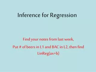
Blood alcohol content (bac) as a function of alcohol consumed (number of beers) for a random sample of 16 adults. What do you predict for 5 beers consumed?What are typical values of BAC when 5 beers are consumed? Give a range.
Conditions for inference • The observations are independent • The relationship is indeed linear (in the parameters) • The standard deviation of y, σ, is the same for all values of x • The response y varies Normallyaround its mean at a given x
Using residual plots to check for regression validity The residuals (y – ŷ) give useful information about the contribution of individual data points to the overall pattern of scatter. We view the residuals in a residual plot: If residuals are scattered randomly around 0 with uniform variation, it indicates that the data fit a linear model, have Normally distributed residuals for each value of x, and constant standard deviation σ.
Residuals are randomly scattered good! Curved pattern the shape of the relationship is not modeled correctly. Change in variability across plotσ not equal for all values of x.
Frog mating call The data are a random sample of frogs. The relationship is clearly linear. The residuals are roughly Normally distributed. The spread of the residuals around 0 is fairly homogenous along all values of x.
Objectives (PSLS Chapter 23) Inference for regression (NHST Regression Inference Award)[B level award]Note Change • The regression model • Confidence interval for the regression slope β • Testing the hypothesis of no linear relationship • Inference for prediction • Conditions for inference