Download
1 / 28
280 likes | 729 Vues
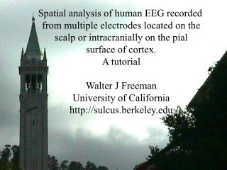
Tutorial on Spatial analysis of human EEG. Spatial analysis of human EEG recorded from multiple electrodes located on the scalp or intracranially on the pial surface of cortex. A tutorial Walter J Freeman University of California http://sulcus.berkeley.edu. Outline. OUTLINE.

E N D
Tutorial on Spatial analysis of human EEG Spatial analysis of human EEG recorded from multiple electrodes located on the scalp or intracranially on the pial surface of cortex. A tutorial Walter J Freeman University of California http://sulcus.berkeley.edu
Outline OUTLINE 1. Review of temporal spectral analysis and spatial spectral analysis of human scalp EEG 2. High resolution spatial pattern discovery using dense arrays of electrodes for EEG scalp recording 3. High resolution spatiotemporal pattern discovery using the Hilbert transform to extract the analytic phase and the instantaneous gamma frequency Walter J Freeman University of California at Berkeley
Time Ensemble Averaging, Evoked potentials In TEA the EEG traces are aligned with the stimulus time marker and summed over N trials at each time point. The amplitude and phase patterns are determined by the stimulus site and the afferent axons. Walter J Freeman University of California at Berkeley
Spatial Ensemble Averaging of EEG “spontaneous” activity In SEA the amplitude and phase are endogenously determined. Phase is defined with respect to the spatial ensemble average wave. Walter J Freeman University of California at Berkeley
Comparing EEG and EMG in temporal and spectral domains From Freeman et al. 2003 Walter J Freeman University of California at Berkeley
Intracranial electrodearrays 1 cm 10x10 cm 1.25 mm 1x1 cm 8x8 8x8 0.5 mm 1x64 32 mm Walter J Freeman University of California at Berkeley
Step One: Spatial sampling vs. spatial function Step One in Spatial EEG Analysis: Electrode design The standard clinical montages are designed to give a spatial sample from the cortex. They are intended to display signals from discrete generators, normal or pathological. Analysis is by Laplacian operators that improve the isolation of the signals. An alternative approach is to search for spatial patterns of EEG activity generated by broad areas of cortex. A different type of array is required: high-density by close spacing of electrodes. The method is implemented by fixing all available electrodes in a line, with spacing that is close enough together to measure the texture of patterns. This procedure is called “over-sampling”. The method is applied to scalp EEG with 64 electrodes spaced at intervals of 3 mm, giving an array that is 189 mm long. Walter J Freeman University of California at Berkeley
Scalp recording with high density linear array A photo montage shows the pial surface of a human brain, projected to the scalp - gyri are light, sulci are dark. EEG were from 64 electrodes. Representative traces are shown of EEG and muscle potentials (EMG). From Freeman et al. 2003 Walter J Freeman University of California at Berkeley
Step Two: temporal spectral analysis Step Two in Spatial EEG Analysis: Temporal spectra Signal analysis in the time domain proceeds by calculation of the power spectral density (PSDt) of the signal, most often by means of the Fast Fourier Transform (FFT). This transformation from the time domain into the temporal frequency domain enables clinicians to detect periodic signals by the peaks they cause in the PSDt. The FFT also helps to determine the optimal rate at which to sample the EEG in analog to digital conversion. The usual criterion is to look for the peaks in the PSDt and choose a cut-off just above the peak with the highest frequency. That cut-off is called the Nyquist frequency. The sample rate must be at least twice the Nyquist frequency and preferably three times higher - The practical Nyquist frequency (Barlow, 1993). Walter J Freeman University of California at Berkeley
Comparison of linear vs. log-log spectral displays The most common display of the power spectral density (PSDt) of EEG time series is in linear coordinates: power vs. frequency. This prevents visualization of the beta and gamma ranges. The display of PSDt as log10 power Vs. log10 frequency shows the form as 1/fa: linear fall-off in log power with increasing log frequency in Hz. The real power is proportional to the square of the frequency. Activity in the gamma band needs substantial metabolic energy. Walter J Freeman University of California at Berkeley
Examples of temporal spectrafrom frontal areas The conventional subdivisions of the EEG spectrum are based on empirical observations, not on brain theory or neurodynamics. From Freeman et al. 2003 Walter J Freeman University of California at Berkeley
Step Three: Spatial spectral analysis Step Three in spatial EEG analysis: Spatial spectral analysis Calculation of the spatial power spectral density PSDx from a curvilinear electrode array is by means of the same mathematical algorithm in space as in time. The interval between electrodes corresponds to the digitizing step in time series signal analysis. The FFT is applied to the 64 amplitudes of EEG at each time step. In practice, the FFT is taken over a 5 s window with 1000 time steps at a sample rate of 200/s (5 ms interval), and the average is computed for the 64 PSDt. Then the FFT is taken over the 189 mm window with 64 samples at a sample rate of 3.33/cm (3 mm interval) and averaged over the 1000 time steps in the same time window. Walter J Freeman University of California at Berkeley
Spatial spectrum of the gyri-sulci & EEG From Freeman et al. 2003 Walter J Freeman University of California at Berkeley
Examples of spatial spectra from the frontal areas Examples from nine subjects show the variability of spatial spectra. From Freeman et al. 2003 Walter J Freeman University of California at Berkeley
Comparison of scalp and intracranial PSDx The pial PSDx is 1/f, but the scalp PSDx is not, due to impedance of dura, skull and scalp, yet a prominent peak persists @ .1-.3 c/cm. From Freeman et al. 2003 Walter J Freeman University of California at Berkeley
Explain the spatial spectral peak at the frequency of gyri A peak can appear in the spatial PSDx of the scalp EEG only if the oscillations over the temporal PSDt are synchronous everywhere in neighboring gyri facing across the sulci. Walter J Freeman University of California at Berkeley
Decomposition of spatial spectra by temporal passband The spatial spectrum is calculated for narrow temporal bands in order to test the hypothesis that oscillations with high temporal frequency are smoothed at high spatial frequency. This dispersion relation is disproved. Instead, the spatial peak in the range of gyral frequency is found in all temporal bands. This implies that an aperiodic temporal pulse with a periodic spatial frequency exists in the scalp EEG. How can it be demonstrated? From Freeman et al. 2003 Walter J Freeman University of California at Berkeley
Step Four:An introduction to cortical state transitions Step Four: An introduction to cortical state transitions Fourier analysis was not appropriate in a search for an event that was temporally aperiodic although it was spatially periodic. The gyral peak was most pronounced when alpha or theta was also present in the unfiltered EEG, that is, when the EEG was also nearly temporally periodic. However, the broad distribution of the spatial spectral spike across the temporal spectrum indicated that the periodic spatial event was a temporal spike, usually occurring aperiodically, but sometimes nearly periodically at alpha-theta rates. The most likely candidate for this occult event was a global, hemisphere-wide state transition, by which cortical dynamics changed abruptly and unpredictably - as in cognition. Walter J Freeman University of California at Berkeley
Step Five: An introduction to the Hilbert transform Step Five: An introduction to the Hilbert transform The most important characteristic of a cortical state transition is the re-initialization of the phase of the on-going oscillations in the beta and gamma ranges of the EEG. Because state transitions may occupy the entire hemisphere, the change in phase can be observed in the scalp EEG, which reflects broad, non-local spatial patterns. Fourier analysis lacks temporal resolution, because it requires the measurement of frequency before phase. The Hilbert transform gives the analytic phase, from which the rate of change in phase gives the instantaneous analytic frequency. Therefore the method of choice for detecting state transitions in the cortical EEG is the Hilbert transform. Walter J Freeman University of California at Berkeley
The Hilbert transform gives high temporal resolution of phase Walter J Freeman University of California at Berkeley
Identification of the optimal pass band before using the HT The Hilbert transform cannot be used without band pass temporal filtering. The identification of optimal high-pass and low-pass settings is by constructing tuning curves to maximize the peak of the cospectrum in the alpha range. From Freeman, Burke & Holmes, 2003
Analytic phase changes abruptly and aperiodically Walter J Freeman University of California at Berkeley
Partial synchronization across the frontal area From Freeman, Burke & Holmes, 2003 Walter J Freeman University of California at Berkeley
Spatial filtering to clarify analytic phase differences From Freeman, Burke & Holmes, 2003 Walter J Freeman University of California at Berkeley
Comparison of CAPD in the beta and gamma ranges From Freeman, Burke & Holmes, 2003 Walter J Freeman University of California at Berkeley
De-periodicization vs. De-synchronization with EMG From Freeman, Burke & Holmes, 2003 Walter J Freeman University of California at Berkeley
References Freeman, W. J. [2000] Neurodynamics. Springer-Verlag. Freeman, W. J. [2001] How Brains Make Up Their Minds. Columbia University Press. Freeman, W. J. [2003] A neurobiological theory of meaning, International Journal of Bifurcation & Chaos, September. Freeman, W. J., Burke, B C., Holmes, M. D. & Vanhatalo, S. [2003] Clinical Neurophysiology 114(6): 1055-1066. Freeman, W. J., Burke, B. C. & Holmes, M. D. [2003] Human Brain Mapping 19: in press. http://sulcus.berkeley.edu References
Acknowledgements Acknowledgments This work was supported by grants to Prof. Robert Kozma from NASA (NCC2-1244) and from NSF (EIA-0130352). EEG and EMG data were collected and edited by Dr. Mark D. Holmes and Dr. Sampsa Vanhatalo, the EEG Clinic of Harborview Hospital, University of Washington, Seattle, and analyzed in the Department of Molecular & Cell Biology, the University of California at Berkeley. Programs were by Linda Rogers and Brian Burke. Prior animal data were collected in collaboration with John Barrie, Mark Lenhart, and Gyöngyi Gaál, and with support by grants from NIMH (MH06686) and ONR (N00014-93-1-09380.