Hydrologic Post-Processor Ensemble Prediction Evaluation Test
Evaluate alternative approaches for generating ensemble predictions of observed streamflows using calibration hydrographs. Focus on period 12/15-2/13. Comparison of streamflow hydrographs, statistics, errors, correlations, and distributions. GLM able to create skillful ensemble members.

Hydrologic Post-Processor Ensemble Prediction Evaluation Test
E N D
Presentation Transcript
NFDC1 Simulation Example Forecast Date 12/15 Nf = 60 days Na = 8 days
Objective • The objective of this test is to evaluate alternative approaches for a hydrologic post-processor to generate an ensemble prediction (simulation) of observed streamflows using calibration hydrographs and corresponding observations as input data. • Focus is on the period 12/15 – 2/13
Example: NFDC1 Dec 15 Select historical data from each year from a window of N days where N = Na + Nf + Nbuffer Analysis Period Future Period Qobsf (to be predicted) Qsimf (given) Qobsa (given) Qsima (given) Time Na = 8 Nf = 60 Nbuffer/2 Nbuffer/2 Nw = Na + Nf “Present” (t = 0) Nbuffer = 30 Note: Nbuffer sets of Nw days of data are taken from each of NYR years of data. This gives NOBS = NYRS * Nbuffer observations for each day
Comparison of Observed, Simulated and Adjusted Ensemble Streamflow Hydrographs (z-space)
Comparison of Observed, Simulated and Adjusted Ensemble Streamflow Hydrographs
Mean and Standard Deviation Statistics of Observed, Simulated and Adjusted Ensemble Members
Correlations between Observed and Simulated and Ensemble Means
Cumulative Distribution Functions of Daily Observed, Simulated and Adjusted Ensemble Streamflow Values
Conclusions • The General Linear Model (GLM) was able to: • Create ensemble members that have the same climatology as the observed values • Preserved “intrinsic” skill (after phase error correction) • Reduces RMS error of raw model simulation • Appears to give reasonable ensemble estimates of Qobs from single-value calibration simulations