Impurity data analysis using UTC
Impurity data analysis using UTC. K-D Zastrow. A tokamak with flux surfaces and a line of sight. Neutrals and ions emit characteristic spectral lines from regions of the plasma where they can exist (“just the right environmental conditions”)

Impurity data analysis using UTC
E N D
Presentation Transcript
Impurity data analysis using UTC K-D Zastrow K-D Zastrow - ADAS Course 2010
A tokamak with flux surfaces and a line of sight Neutrals and ions emit characteristic spectral lines from regions of the plasma where they can exist (“just the right environmental conditions”) Electrons and ions follow field lines that map out a flux surface defined by constant pressure (pe+pi). Transport along a field line is fast, transport perpendicular to it is slow. As a result, temperatures and densities are themselves constant on flux surfaces. The 3D transport problem is reduced to 1D by use of a flux surface label as radial co-ordinate. K-D Zastrow - ADAS Course 2010
Example Ni - Coronal balance? Coronal f(Niq+) is function of Te.Te is function of r. f(Niq+) is also a function of r. But is it given by Te(r) as shown here? K-D Zastrow - ADAS Course 2010
Timescales for transport and atomic processes Emission neX 1020 m-3 10-12 m3/s 108/sec Ionisation neS 1020 m-3 10-14 m3/s 106/sec Diffusion D/(0.1 a)2 1 m2/sec / 0.01m2 100/sec Convection v/(0.1 a) 1 m/sec / 0.1m 10/sec Recombination ne 1020 cm-3 10-20 m3/s 1/sec • Emission is a local process • Timescale for transport is slower than ionisation but faster than recombination, therefore density profile of individual ionisation stage is determined non-locally K-D Zastrow - ADAS Course 2010
Equations for particle transport The “standard model” Particle conservation with empirical ansatz for Z Task: measure DZ(r,t), vZ(r,t). Turn photon fluxes into densities. Sources and sinks Z(r,t) : electron and neutral collisions K-D Zastrow - ADAS Course 2010
Some comments on the edge model • For r/a>1.0 the code (SANCO) also requires parameters for calculations • Electron temperature and density • Neutral particle source rate 0(t) • Neutral particle velocity for influx mean free path • SOL loss rate given by parallel confinement time -nZ/|| • Diffusion and convection continue from last defined value in the core • Recycling coefficient (not recommended…) • These parameters are all meaningless and should not be interpreted as physics results. • The only thing that’s meaningful is the outermost measurement (whatever it is) and how well this is matched. • It is worth checking that a change in these parameters does not affect the results in the core. • Change in particle velocity will change required influx rate but should change nothing else within reason • SOL density, temperature and particle velocity should combine so that the SOL is easily penetrable • Parallel loss rate, DSOL and vSOL should combine to a perfect sink K-D Zastrow - ADAS Course 2010
The ambiguity problem in steady-state • Steady state profile shape in source free region given by • Same solution obtained for 20, 2D and 2v etc. • We need transient experiments to resolve D and v separately K-D Zastrow - ADAS Course 2010
Sensitivity study Testing against data Three types of impurity transport modelling • Measurement of concentration or influx from spectroscopic observations • Impurity transport code is needed for interpretation but transport coefficients cannot be derived. • Measurement of impurity transport coefficients • Coefficients in an empirical ansatz with diffusion and convection are fitted to data (success criteria?) • Integrated plasma modelling including impurities • Theory based or empirical expressions are used, the main interest is to predict dilution and radiative power as well as other more exotic effects. K-D Zastrow - ADAS Course 2010
Choosing data to fit against • A short time window after a gas puff (laser blow off, ELM, sawtooth crash….) carries transient information, so D can be determined from the relaxation of the profile. • Often not enough data to determine both v and D. • A long quasi steady-state time window gives good statistics to determine v/D, as well as data on recycling from rate of decay. • Ambiguity problem. • The choice of time window will not only influence the accuracy of the results but also what exactly is measured. K-D Zastrow - ADAS Course 2010
Usable data and modelling needs K-D Zastrow - ADAS Course 2010
Parameterise coefficients D(r,t), v(r,t), 0(t) Model all data and adjust parameters by eyeballing Estimate data errors, calculate 2 Least squares fit Generate derivatives by changing one parameter at a time Improve solution using covariance (Levenberg-Marquardt Method) Confronting data and model K-D Zastrow - ADAS Course 2010
Practicalities of fitting a model • The fitting program (UTC) is a wrapper that generates input files for a transport code (SANCO) and collects the output files. • UTC executes all post processing, including instrumental time and space resolution. • For each data point UTC generates a value from the model and derivatives with respect to each fit parameter. • UTC operates on the “house number” of the data point, where each data point has a weight. K-D Zastrow - ADAS Course 2010
Levenberg-Marquardt Method • Data point house number n • Data vector y • Model vector f described by parameter vector p • Co-variance matrix M • Improve solution by changing p iteratively • Far from the solution, ignore co-variance terms and slow down rate of improvement change by multiplying diagonal of M • In every iteration, try several damp factors d and pick the best • For every iteration, damp factor should be decreased to optimise speed K-D Zastrow - ADAS Course 2010
Model parameterisation • D and v on a radial and time grid. • Analogy: diagnostic with finite resolution. • Practical number of grid points depends on the resolution of the data. • Fit will not converge if information is not present in the data. • The model needs parameters in regions where there are no measurements D t=[t1,t2] t=[t2,t3] r v K-D Zastrow - ADAS Course 2010
Errors of transport parameters • Covariance of errors in fit parameters returned. If large then both parameters do the same job (ambiguity) • Assumes 2N-m. • Assumes model and weights to be correct • Errors (weights) are taken to be uncorrelated. For correlated errors a UTC extension exists but is not part of the code • Same matrix as in least squares fit but without damp factor (1+d2) in Levenberg-Marquardt K-D Zastrow - ADAS Course 2010
What UTC and SANCO need from the user • Plasma background data (Te(), ne()) • Plasma geometry • Mapping local parameters () on lines of sight (x,y,z) • Plasma volume changes with radius • Diagnostic information • What is measured (physics, ADAS) • What are the instrumental parameters (sensitivity, geometry, time and space resolution) • Transport model parameterised – influx, core and edge transport including “nuisance” parameters K-D Zastrow - ADAS Course 2010
UTC and SANCO on other fusion plasmas but JET? • SANCO is a stand alone code. Only reads and writes files. • UTC interface with JET is through a small number of data access routines that need changing • Already converted for MAST by A Foster K-D Zastrow - ADAS Course 2010
Tutorial session • Not enough time in one day to go through it all if we start from scratch • Two cases prepared so you can see the result and start to use the interfaces • Estimate impurity concentration from line integrated data • Derive v and D from Neon puff experiment • Hopefully illustrate sensitivity studies and limitations • Hopefully illustrate efficiency once everything is set up • To start with, demonstrate the menus and what they do • Real transport studies requires good understanding of the data being analysed, as well as careful thought and analysis. We are not going to get “final” answers today! K-D Zastrow - ADAS Course 2010
Just before we go for lunch… • Set up you account • Include /u/cxs/utc/code in your IDL path • If you haven’t already got one, create a .netrc file with one line • “machine ppfhost login YOURID password YOURPW” • Then to prevent others reading your password >chmod 600 .netrc • Copy files from my space • /u/kdz/adascourse/* > idl > utc - then load a .utc file • If it works, go for lunch • Tutorials start when we re-convene • If it doesn’t, we need to sort it out first K-D Zastrow - ADAS Course 2010
Exercises • 73576 (Ni) • Define a graph that shows radial profiles of ionisation stages. Explore changes in these with changing transport coefficients. • Explore the effect of the edge model parameters on the solution. • Why is the simulated Ni signal not constant in time? • 60932 (Ne) • Optimising the transport parametrisation • Developing a better influx model • Understanding the co-variance matrix – to fit or not to fit • Gradual approach to final solution • Time permitting • Start from scratch for a different impurity and/or shot K-D Zastrow - ADAS Course 2010
Appendix K-D Zastrow - ADAS Course 2010
2 with correlated errors Matrices can and will become very big! Reverts to standard definition of 2 if errors are not correlated K-D Zastrow - ADAS Course 2010
Errors in fixed model parameters Treat as if the error is a property of the data One non-fitted model parameter Different electron temperature K-D Zastrow - ADAS Course 2010