Nonparametric hidden Markov models
Nonparametric hidden Markov models. Jurgen Van Gael and Zoubin Ghahramani. Introduction. HM models: time series with discrete hidden states Infinite HM models ( iHMM ): nonparametric Bayesian approach Equivalence between Polya urn and HDP interpretations for iHMM

Nonparametric hidden Markov models
E N D
Presentation Transcript
Nonparametrichidden Markov models Jurgen Van Gael and ZoubinGhahramani
Introduction • HM models: time series with discrete hidden states • Infinite HM models (iHMM): nonparametric Bayesian approach • Equivalence between Polya urn and HDP interpretations for iHMM • Inference algorithms: collapsed Gibbs sampler, beam sampler • Use of iHMM: simple sequence labeling task
Introduction • Underlying hidden structure examples • Observed pixels corresponding to objects • Power-spectra coefficients on a speech signal corresponding to phones • Price movements of financial instruments corresponding to underlying economic and political events • Models with such underlying hidden variables can be more interpretable and better predictive properties than models directly relating with observed variables • HMM assumes 1st order Markov properties on the Markov chain of hidden variables with a KxK transition matrix • Observation depends usually on an observation model F parameterized by a state-dependent parameter • Choosing the number of states K: nonparametric Bayesian approach for hidden Markov model with countably infinite number of hidden states
From HMMs to Bayesian HMMs • An example of HMM: speech recognition • Hidden state sequence: phones • Observation: acoustic signals • Parameters , come from a physical model of speech / can be learned from recordings of speech • Computational questions • 1.(, , K) is given: apply Bayes rule to find posterior of hidden variables • Computation can be done by a dynamic programming called forward-backward algorithm • 2. K given, , not given: apply EM • 3 .(, , K) is not given: penalizing, etc..
From HMMs to Bayesian HMMs • Fully Bayesian approach • Adding priors for , and extending full joint pdfas • Compute the marginal likelihood or evidence for comparing, choosing or averaging over different values of K. • Analytic computing of the marginal likelihood is intractable
From HMMs to Bayesian HMMs • Methods for dealing the intractability • MCMC 1: by estimating the marginal likelihood explicitly. Annealed importance sampling, Bridge sampling. Computationally expensive. • MCMC 2: by switching between different K values. Reversible jump MCMC • Approximation by using good state sequence: by independency of parameters and conjugacy between prior and likelihood under given hidden states, marginal likelihood can be computed analytically. • Variational Bayesian inference: by computing lower bound of the marginal likelihood and applying VB inference.
Infinite HMM – hierarchical Polya Urn • iHMM: Instead of defining K different HMMs, implicitly define a distribution over the number of visited states. • Polya Urn: • add a ball of new color: / (+ni). • add a ball of color i : ni/ (+ni). • Nonparametric clustering scheme • Hierarchical Polya Urn: • Assume separate Urn(k) for each state k • At each time step t, select a ball from the corresponding Urn(k)_(t-1) • Interpretation of transition probability by the # of balls of color j in Urn color i: • Probability of drawing from oracle:
HDP and hierarchical Polya Urn • Set rows of transition matrix equal to the sticks of Gj • Gj corresponds to the Urn for the j-th state • Key fact: all Urns share the same set of parameters via oracle Urn
Inference • Gibbs sampler: O(KT2) • Approximate Gibbs sampler: O(KT) • State sequence variables are strongly correlated slow mixing • Beam sampler as an auxiliary variable MCMC algorithm • Resamples the whole Markov chain at once • Hence suffers less from slow mixing
Inference – collapsed Gibbs sampler • Given and s1:T, the DPs for each transition becomes independent (?) • By fixing s1:T, the j-th state does not depend on the previous state • could be marginalized
Inference – collapsed Gibbs sampler • Sampling st: • Conditional likelihood of yt: • Second factor: a draw from a Polya urn
Inference – collapsed Gibbs sampler • Sampling : from the Polya Urn of the base distribution (oracle Urn) • mij : the number of oracle calls for a ball with label j when queried the oracle from state i. • Note: use for sampling • :# of transitions from i to j . • mij: # of elements in Sij that were obtained from querying the oracle. • Complexity: O(TK+K*K) • Strong correlation of the sequential data: slow mixing behavior
Inference – Beam sampler • A method of resampling the whole state sequence at once • Forward-filtering backward-sampling algorithm does not apply because of the number of states and hence the number of potential state trajectories is infinite • Introducing auxiliary variables • Conditioned on , the number of trajectories is finite • These auxiliary variables do not change the marginal distributions over other variables hence MCMC sampling still converges to the true posterior • Sampling and : • k = ~ • Each k is independent of others conditional on and
Inference – Beam sampler • Compute only for finitely many st, st-1 values.
Inference – Beam sampler • Complexity: O(TK2) when K states are presented • Remarks: auxiliary variables need not be sampled from uniform. Beta distribution could also be used to bias auxiliary variables close to the boundaries of
Example: unsupervised part-of–speech (PoS) tagging • PoS-tagging: annotating the words in a sentence with their appropriate part-of-speech tag • “ The man sat” ‘The’ : determiner, ‘man’: noun, ‘sat’: verb • HM model is commonly used • Observation: words • Hidden: unknown PoP-tag • Usually learned using a corpus of annotated sentences: building corpus is expensive • In iHMM • Multinomial likelihood is assumed • with base distribution H as symmetric Dirichlet so its conjugate to multinomial likelihood • Trained on section 0 of WSJ of Penn Treebank: 1917 sentences with total of 50282 word tokens (observations) and 7904 word types (dictionary size) • Initialize the sampler with 50 states with 50000 iterations
Example: unsupervised part-of–speech (PoS) tagging • Top 5 words for the five most common states • Top line: state ID and frequency • Rows: top 5 words with frequency in the sample • state 9: class of prepositions • State 12: determinants + possessive pronouns • State 8: punctuation + some coordinating conjunction • State 18: nouns • State 17: personal pronouns
Beyond the iHMM: input-output(IO) iHMM • MC affected by external factors • A robot is driving around in a room while taking pictures (room index picture) • If robot follows a particular policy, robots action can be integrated as an input to iHMM (IO-iHMM) • Three dimensional transition matrix:
Beyond the iHMM: sticky and block-diagonal iHMM • Weight on the diagonal of the transition matrix controls the frequency of state transitions • Probability of staying in state i for g times: • Sticky iHMM: by adding a prior probability mass to the diagonal of the transition matrix and applying a dynamic programming based inference • Appropriate for segmentation problems where the number of segments is not known a priori • To carry more weight for diagonal entry: • is a parameter for controlling the switching rate • Block-diagonal iHMM:for grouping of states • Sticky iHMM is a case for size 1 block • Larger blocks allow unsupervised clustering of states • Used for unsupervised learning of view-based object models from video data where each block corresponds to an object. • Intuition behind: Temporary contiguous video frames are more likely correspond to different views of the same objects than different objects • Hidden semi-Markov model • Assuming an explicit duration model for the time spent in a particular state
Beyond the iHMM:iHMM with Pitman-Yor base distribution • Frequency vs. rank of colors (on log-log scale) • DP is quite specific about distribution implied in the Polya Urn: colors that appear once or twice is very small • Pitman-Yor can be more specific about the tails • Pitman-Yor fits a power-law distribution (linear fitting in the plot) • Replace DP by Pitman-Yor in most cases • Helpful comments on beam sampler
Beyond the iHMM: autoregressive iHMM, SLD-iHMM • AR-iHMM: Observations follow auto-regressive dynamics • SLD-iHMM: part of the continuous variables are observed and the unobserved variables follow linear dynamics SLD model FA-HMM model

