Download
1 / 24
240 likes | 402 Vues
Testify and Constrain the Flare Model Using RHESSI observations. Jin Meng NJU SOLAR GROUP 2007.10.18. Standard flare model. Study1: A statistical study about asymmetry and correlation. RHESSI (Lin et al. 2002). Yohkoh (Sakao, 1994; Masuda, 1994). SMM (Brown, 1971)

E N D
Testify and Constrain the Flare Model Using RHESSI observations Jin Meng NJU SOLAR GROUP 2007.10.18
Standard flare model Study1: A statistical study about asymmetry and correlation RHESSI (Lin et al. 2002) Yohkoh (Sakao, 1994; Masuda, 1994) SMM (Brown, 1971) Hinoatori (Petrosian, 1973) Study2: An evidence of chromospheric evaporation
Observed Asymmetrical Footpoints Yohkoh observation of 1991 December 26 flare RHESSI observation of 2005 January 15 flare Yohkoh/SXT Yohkoh/HXT (Li et al. 1997) (Jin & Ding 2007)
Variations of the hard X-ray footpoint asymmetry in a solar flare (Siarkowski et al. 2004)
A statistical study • The asymmetries of hard X-ray footpoints for 29 solar flares observed by RHESSI in 2002-2005. • The correlations of hard X-ray footpoints. • Using Fourier Method to divide the fluxes into slowly-varying components and fast-varying components and test their correlations seperately.
Observations and selection of samples Samples: 29 flares (3 C-class, 18 M-class, 8 X-class) Hard X-ray contours for 6 RHESSI flares, overlaid on the magnetograms observed by SOHO/MDI. The blue, red, and yellow contours represent 25–50, 50–100, 100–300 keV, respectively. The green lines represent the magnetic neutral lines.
RHESSI images of the 2005 January 5 flare at 00:26:20 UT • Data analysis • Asymmetry of footpoints • F1-F2/F1+F2 • Hard X-ray light curves • Method: CLEAN • The integration time 8 s • Correlation of footpoints • Slowly-varying components: >32 s • Fast-varying components: 8-32 s Hard X-ray light curves at 50–100 keV of the 2005 January 5 flare at 00:26:20 UT
Results The correlation coefficients of the slow components are usually high. For fast components, the majority of them show low correlation coefficients. The data points for 50-100 keV are slightly more dispersed, possibly because of more noise in the higher energy band. Footpoint correlation coefficients of slowly varying components versus that of fast varying components
Results The footpoint asymmetries vary from case to case. However, the footpoint correlations are always high regardless of whatever asymmetries there are. There are very few exceptions, in the 50-100 keV band, in which the correlation is weak. Asymmetries versus correlation coefficients of flare footpoints
Discussion 1Interpretations about asymmetries • The mirroring effect (e.g., Sakao 1994; Aschwanden et al. 1999) • Asymmetric magnetic reconnection • Emslie et al. (2003) found evidence of the differentcolumn densities implied by a difference in spectral indices of the footpoints. • Through numerical calculations, Falewicz & Siarkowski (2007) found that an asymmetric electron injection site, together with different mass densities in the loop, can quantitatively account for the observed hard X-ray asymmetries. Recent observations showed that such a scenario is not always true (Asai et al. 2002; Goff et al. 2004)
Discussion 2Interpretations about correlations • Fine time structures in solar flare emission • HXR emission(e.g., Kiplinger et al. 1983, 1984; Dennis 1986; Aschwanden et al. 1995, 1998) • Mictrowave emissions (e.g., Slottje 1978; Takakura et al. 1983; Elgaroy 1986; Kliem et al. 2000; Nakajima 2000) • Optical emissions (Wang et al. 2000; Ding et al. 2001; Ding 2005) They are all thought to be related to the time characteristics of electron beams
Discussion 2Interpretations about correlations • An assumption is that the fine structures in the hard X-ray time profile correspond to small-scale electron injections, and that the slow components are build up by a large number of such small bursts. • Low correlation between the fast hard X-ray components imply that the injections are not evenly distributed along the two legs. • High correlation between the slow components suggest that the time integrations of such injections, on long timescales, are still correlated. Such a scenario is consistent with a turbulent model proposed by Jakimiec (1998)
Conclusions • There is usually a good correlation between the light curves of the two conjugate footpoints in a flare. However, the correlations for the slow components are much betterthan those for fast components. • Asymmetries between hard X-ray footpoints are a common phenomenon in solar flares. However, in most asymmetric cases, the correlations between the footpoints remain high. • The results suggest a scenario that the small injections of electrons are independent in the two footpoints, while the integration of them (revealed by the slow component in the light curve) still keeps a high correlation. Back to standard flare model
Observation evidence of chromospheric evaporation Left: An EUV Imaging Telescope (EIT) 195A image showing a post-flare loop on 19 January 2005. Right: A velocity map taken from the same region using the Fe XIX (~8 MK) emission line as observed by CDS. (Ryan Milligan, 2007, RHESSI Nuggets) Strong blueshifts are clearly visible at the HXR footpoints as observed by RHESSI Centroids of the northern and southern halves of the loop at different energies for the three 24-second time intervals (Liu, et al. 2006)
Loop-like HXR emission in the 20 January 2005 Flare Reconstructed hard X-ray images using different methods and time intervals. The energy band is 25-50 keV for all the three maps.
SOHO/MDI & EIT images SOHO/MDI magnetograms at 05:46:02 UT EIT 195A image at 06:48:12 UT
Evolution of hard X-ray sources in 25-50 keV Phase I: a-d The two FPs clearly appear while the LT is invisible in this period. Phase II: e-f The LT source appears. Phase III: g-l The emission from the legs of the loop appears. The LT source dominates progressively. Phase IV: m-p The emission from the LT is dominant in this phase.
Light curves of the event RHESSI lightcurves of the flare on 2005 January 20 Lightcurves of different hard X-ray sources
A estimate about the velocity of upflows using lightcurves: 150 km/s Recent observation using SOHO/CDS reported 140-200 km/s in FeXIX (Del Zanna & Mason 2005)
Evolution of spectral indices of different hard X-ray sources • We find that the power-law indices of the two FPs are very close and show a clearly soft-hard-soft behavior. • It is clear that spectra in the loop legs and the LT are softer than in the FPs. • The power-law indices have a tendency to become softer during the stage when the loop emission is visible. Energy band for fitting For two FPs: 29.5-56 keV For LT and Legs: 16-24 keV The two vertical dotted lines show the time period when the loop-like HXR emission is visible in 25-50 keV RHESSI images
Discussion The general picture of the 2005 January 20 flare: Magnetic reconnection (impulsive phase of the flare) non-thermal electrons travel from corona to the chromosphere HXR emission through thick-target bremsstrahlung the released energy heats the chromospheric material upward mass motion in the loop the density in the loop is large enough for thick-target bremsstrahlung Loop show HXR emission quasi-stationary state in the loop light curves show a plateau in the loop A Cartoon of the basic model of chromospheric evaporation (RHESSI Nuggets)
Remarks • The loop-like HXR emission reported for the 2005 January 20 flare is helpful for us to understand the physical processes in the loops of flares. • A theoretical approach that incorporates the chromospheric evaporation and the production of HXR emission is desired in the near future to interpret such an observational result.
Thank you! Děkujivam!