Hinode AR and Flare Observations

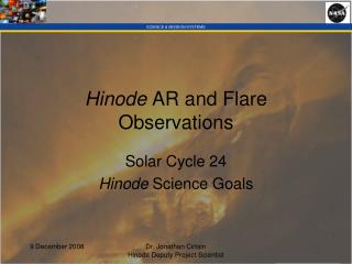
1. Hinode AR and Flare Observations Solar Cycle 24 Hinode Science Goals Dr. Jonathan Cirtain Hinode Deputy Project Scientist

2. Overview • Hinode AR and Flare past Observations • Hinode AR and Flare planning • Capabilities • AR observation plans • Flare Observation plans • External Requests • Data Access Dr. Jonathan Cirtain Hinode Deputy Project Scientist

3. Hinode Active Region Observations • EIS slot movies (w/raster) provide unique opportunities to observe flares (40” & 240”) Dr. Jonathan Cirtain Hinode Deputy Project Scientist

4. Hinode Active Region Observations • NFI/SOT is capable of making high-cadence high resolution line-of-sight magnetograms Dr. Jonathan Cirtain Hinode Deputy Project Scientist

5. Hinode Active Region Observations BFI/SOT: Can make high cadence high-resolution images in visible and near UV Dr. Jonathan Cirtain Hinode Deputy Project Scientist

6. Hinode Flare Observations XRT has only made a few flare observations, but they are really impressive! Dr. Jonathan Cirtain Hinode Deputy Project Scientist

7. Flare Mode of Operation • Each instrument is capable of response to a flare • XRT can take Flare Patrol images on a pre-specified cadence • Once the flare flag is raised XRT, SOT, and EIS can change to a designated flare program • SOT can use the FPI to determine the position of the flare and center on that region! • XRT can store pre-flare data in a special buffer Dr. Jonathan Cirtain Hinode Deputy Project Scientist

8. XRT Active region planed observations • Temperature • Multiple filter observations • Topology • High resolution with moderate FOV and 1-3 filters • Dynamics • High cadence (10-30 sec btw images) and single filter Dr. Jonathan Cirtain Hinode Deputy Project Scientist

9. EIS Active Region Planned Observations • Sit & Stare • Large line list with Fe VIII – Fe XXIV coverage (some lines missing) • Ca XIV, XV, XVI • Density sensitive lines at several different peak formation temperatures • Many lines formed from 0.1—1 MK (Mg, Si, O, Ne) for elemental fractionation measurements. • Slit + Slot • Unique EIS observing technique provides context imagery over several different narrow passbands • Line list is reduced in most cases • Other Dr. Jonathan Cirtain Hinode Deputy Project Scientist

10. EIS Flare Planned Observations • Sit and Stare • “Picket Fence” • Fe XII, XV, XVII, XXIII, XIV (2) • Ca XVII • He II (25.6 nm) • 5s exposures, 1 minute raster cadence • Slot (Slot + slit) Dr. Jonathan Cirtain Hinode Deputy Project Scientist

11. EIS Observation of a limb flare Dr. Jonathan Cirtain Hinode Deputy Project Scientist

12. SOT Instrumentation/Capabilities Broadband Filter Imager • Field of view 218" × 109" (full FOV) • CCD 4k × 2k pixel (full FOV), shared with the NFI • Spatial Sampling 0.0541 arcsec/pixel (full resolution) Spectral coverage Center (nm) Band width (nm) Line of interest Purpose 388.35 0.7 CN I Magnetic network imaging 396.85 0.3 Ca II H Chromospheric heating 430.50 0.8 CH I Magnetic elements 450.45 0.4 Blue continuum Temperature 555.05 0.4 Green continuum Temperature 668.40 0.4 Red continuum Temperature Exposure time 0.03 - 0.8 sec (typical) Dr. Jonathan Cirtain Hinode Deputy Project Scientist

13. SOT Instrumentation/Capabilities Narrowband Filter Imager (NFI) • Field of view 328"×164" (unvignetted 264"×164") • CCD 4k×2k pixel (full FOV), shared with BFI • Spatial sampling 0.08 arcsec/pixel (full resolution) • Spectral resolution 0.009nm (90mÅ) at 630nm • Spectral windows (nm) and lines of interest Center Tunable range Lines Purpose 517.2 0.6 Mg I b 517.27 Chromospheric Dopplergrams and magnetgrams 525.0 0.6 Fe 524.71 Photospheric magnetograms 557.6 0.6 Fe I 557.61 Photospheric Dopplergrams 589.6 0.6 Na I D 589.6 Very weak fields (scattering polarization) Chromospheric fields 630.0 0.6 Fe I 630.15 Photospheric magnetograms Fe I 630.25 2.50 Ti I 630.38 0.92 Umbral magnetograms 656.3 0.6 H I 656.28 Chromosphreic structure Exposure time 0.1 - 1.6 sec (typical) Dr. Jonathan Cirtain Hinode Deputy Project Scientist

14. SOT Instrumentation/Capabilities Stokes Polarimeter • Field of view along slit 164" (north-south direction) • Spatial scan range ±164" • Slit width 0.16" • Spectral coverage 630.08nm - 630.32nm • Spectral resolution / sampling 30mÅ / 21.5mÅ • Measurement of polarization Stokes I,Q,U,V simultaneously with dual beams (orthogonal linear components) • Polarization signal to noise 103 (with normal mapping) Dr. Jonathan Cirtain Hinode Deputy Project Scientist

15. SOT Flare Planned Observations • Determine photospheric signatures of energy storage and trigger process that leads to flares. • Shearing motion of magnetic field ⇒ Time series of magnetic field vector data (SP) for 24 hours • Magnetic emergence and disappearance ⇒ Time series of magnetogram & dopplergram (FG:NFI Na) • Determine the coronal configuration(s) of flare sites. • Magnetic field vector data (SP) • Ca II H (Hα is preferred) image (chromospheric structure) Dr. Jonathan Cirtain Hinode Deputy Project Scientist

16. SOT Flare Planned Observations • Capture the temporal evolution of filament eruption as the trigger of flares and arcade structure of flares. • Ca II H image, only applicable to the limb observations • Capture the temporal evolution of filament eruption as the trigger of flares and arcade structure of flares. • Ca II H (chromosphere) and G-band (photosphere) images Dr. Jonathan Cirtain Hinode Deputy Project Scientist

17. SOT standard programs for flare studies Dr. Jonathan Cirtain Hinode Deputy Project Scientist

18. External Requests • Planning for Hinode operations is performed on a three month cycle that is updated monthly. At the end of every month a monthly meeting is held to confirm the observations for the coming month and to lay out the broad objectives for the second and third months. • The cut-off for consideration is the 14th day of each month. For example, requests for observations received between the 15th of June and the 14th of July will be presented and discussed at the monthly meeting held at the end of July. • It is recommended that proposers make their submissions as early as possible, so that the Science Schedule Coordinators (SSCs) have time to refine the proposals to fit the current Hinode situation. • Late submissions may be considered only exceptionally, if scheduling conflicts can be easily resolved in the operation planning meetings. Dr. Jonathan Cirtain Hinode Deputy Project Scientist

19. Information required in submitted proposals • Title of the proposed observation. • Short statement describing the observation, and scientific justification. • This should be as short and concise as possible, but it should still contain all the key details. This statement is important because Hinode's limited data volume situation may make it necessary to modify some planned observations on some days. The Hinode team will refer to this statement when setting priorities for which observations to perform. • Point of contact. Name and email address. • Time period of proposed observations, if required. • Provide the start and end dates with the reason. • Provide the minimum number of observation days during the period. • Provide desires and requirements for continuity of observations, for example: ``three consecutive days are desired, but not required,'' ``three consecutive days are required,'' or ``it is not necessary for observations to be on consecutive days.'' • Time window in day, if required. • Provide the ``minimum'' duration with the start and end times in UT, if it is a coordinated observation with ground-based or space-based observatories. • Specify whether any short interruptions (e.g., for ten-minute synoptics) are allowed over the observing periods. Dr. Jonathan Cirtain Hinode Deputy Project Scientist

20. Information required in submitted proposals cont. • Target of interest. • Clearly specify the target of interest. • Active region, quiet Sun, on-disk, near limb, limb, polar region, etc. • More specific description of the target, if required. • Indicate whether it is a target of opportunity (TOO). If so, suitably describe the target. • If a suitable target does not exist during the specified period, we may not perform the proposed observation during that period. • Required Hinode instruments, and priority of observables. • The Hinode team will take into account the stated priorities if it is necessary to make adjustments to the proposed observations to fit in the day's available telemetry, etc. • Specify which Hinode instruments are really required for the observation. • Specify required observables (cadence, FOV vs pixel summation, wavelengths etc), with priorities, for the primary required Hinode instrument(s). • Provide rough estimate of the total data volume to be collected, if possible. See section 3 for estimating the total data collected. • If support from non-primary Hinode instrument(s) is also desired, give a rough idea regarding preferable observables (cadence, FOV vs pixel summation, wavelengths etc). Dr. Jonathan Cirtain Hinode Deputy Project Scientist

21. Types of suggested HOP observations • Coordinated observations with ground-based facilities and space-borne instruments, if the period/time specification is critical. • Coordination among more than two Hinode instruments if there is a critical time constraint to the observations, or if both instruments are required to consume significant telemetry resources. • Observations requiring telemetry volumes which are a large percentage of the regular allocations of the instruments. Dr. Jonathan Cirtain Hinode Deputy Project Scientist

22. The XRT HOP request form • http://solar.physics.montana.edu/HINODE/XRT/joppelganger.html • Chief Coordinators • John M. Davis (john.m.davis (at) nasa.gov) • Tetsuya Watanabe (watanabe (at) uvlab.mtk.nao.ac.jp) • Scientific Schedule Coordinators - Instrument Specific • Solar Optical Telescope (SOT) • Tom Berger (berger (at) lmsal.com) • Takashi Sekii (sekii (at) solar.mtk.nao.ac.jp) • X-Ray Telescope (XRT) • Leon Golub (Golub (at) head.cfa.harvard.edu) • Kiyoto Shibasaki (shibasaki (at) nro.nao.ac.jp) • EUV Imaging Spectrometer (EIS) • Len Culhane (jlc (at) mssl.ucl.ac.uk )  • Tetsuya Watanabe (watanabe (at) uvlab.mtk.nao.ac.jp ) • John Mariska (mariska (at) nrl.navy.mil ) Dr. Jonathan Cirtain Hinode Deputy Project Scientist

23. Hinode Data Access • http://darts.isas.jaxa.jp/hinode/top.do • http://sdc.uio.no/sdc/welcome • http://sot.lmsal.com/Data.html • http://xrt.cfa.harvard.edu/DATA • http://msslxr.mssl.ucl.ac.uk:8080/SolarB/SearchArchive.jsp Dr. Jonathan Cirtain Hinode Deputy Project Scientist