Map Scale and Projection

Map Scale and Projection

Map Scale and Projections • Map scale and transformations • Distortions resulting from map transformations • Analysis and visualisation of distortion • Choosing a map projection • Commonly used map projections For details about the contents of this topic, please refer to Peter H. Dana, 1999: Map Projection Overview, (http://www.colorado.edu/geography/gcraft/notes/mapproj/mapproj_f.html). Map Scale and Projections

Map scale and transformations • Map, to be useful, are necessarily smaller than the areas mapped. • Map scale - the ratio between measurements on the map to those on the earth. • Transformation from globe to map means that the map’s scale will vary from place to place. Map Scale and Projections

Globe and a flat map Comparison between globe and flat map of the earth. From Robinson, et al., 1995 Map Scale and Projections

Map Scale 1:1,000,000 10 8 6 4 2 0 10 20 30 40 km Statements of scale • Representative fraction (RF): a simple ratio (e.g. 1:20,000) • Verbal statement • Graphical or bar scale (scale bar) Represents 1 km2 Map Scale and Projections

Scale factor • The scale factor (SF) at a point is computed by: • On the reference globe, SF = 1. • As the earth is essentially spherical, while the view represented by a map is orthogonal, the SF will be various from place to place. • The sphere and the plane are not applicable. Map Scale and Projections

i’ h’ i h g’ g f’ f e’ e d’ d c’ c b' b 90° a Scale factor of distance Orthographic projection of an arc to a tangent straight line. After Robinson, et al., 1995 Map Scale and Projections

b b c c a b’ b’ c’ d c’ a d Scale factor of direction Projection of rectangle abcd to rectangle ab’c’d with side ad held constant. Left: the perspective view shows the geometric relations of the two rectangles. Up: the relation of the two rectangles when they are each viewed orthogonally. After Robinson, et al., 1995 Map Scale and Projections

Distortions resulting from map transformations • Whenever the spherical surface is transformed to a plane, it is certain that all of the geometrical relationships on the sphere cannot be entirely duplicated. • The major alternations have to do with angles, areas, distances and directions. Map Scale and Projections

B” B M M’ B’ b U U’ A’ a A 0 P’ P Tissot’s indicatrix • OA = OB = 1.0 • For the ellipse • OA’ = a = 1.25 • OB’ = b = 0.80 • For the dashed • OA’ = a = 1.25 • OB” = b = 1.25 •  = U - U’ Map Scale and Projections

Transformation The great circle (solid line) and the rhumb (dashed line) as they appear on Mercator’s projection. From Robinson, et al., 1995 Map Scale and Projections

Analysis and visualisation of distortion Evaluation of visual characteristics of the earth’s coordinate systems • Parallels are parallel. • Parallels are spaced equally on meridians. • Meridians and great circles on a globe appear as straight lines. • Meridians converge toward the poles and diverge toward the equator. • Meridians are equally spaced on the parallels, but their spacing decreases to the pole. Map Scale and Projections

Analysis and visualisation of distortion (cont.) Evaluation of visual characteristics of the earth’s coordinate systems • Meridians and parallels are equally spaced at or near the equator. • Meridians at 60° latitude are half as far apart as parallels. • Parallels and meridians always intersect at right angles. • The surface area bounded by any two parallels and two meridians is the same anywhere between the same parallels. Map Scale and Projections

Visual analyses Equatorial Oblique Polar Different centerings of the sinusoidal projection produce different appearing graticules. Nevertheless, the arrangement or pattern of the deformation is the same on all, since the same system of transformation is employed. From Robinson, et al., 1995 Map Scale and Projections

Graphical portrayal of distortions A head drawn on the Mollweide projection (top) has been transferred to Mercator’s projection (centre) and to the cylindrical equal-area projection with standard parallels at 30° (bottom). From Robinson, et al., 1995 Map Scale and Projections

Distortions of directions Selected great circle arcs on an equatorial case of the sinusoidal projection showing their departures from straight lines. Each uninterrupted and interrupted arc is 150° long. Courtesy W.R. Tobler, cited in Robinson, et al., 1995 Map Scale and Projections

Choosing a map projection • Cartographers need to be thoroughly familiar with map projections. • Cartographers frequently transfer data from one projection to another. Map Scale and Projections

Guidelines • Projection’s major property: • conformality, equivalence, azimuthality, reasonable appearance, etc. • Amount and arrangement of distortion: • Mean distortion (angular or area). • Map series have special projection requirements. • To show the same pattern of distortion for large areas as for small areas. • The overall shape of the area. Map Scale and Projections

Common distortion patterns on map projection Azimuthal patterns of deformation. (a) The pattern when the plane is tangent to the sphere at a point, and (b) the pattern when the plane intersects the sphere. Conical patterns of deformation. (a) The pattern when the cone is tangent to one small circle, and (b) the pattern when the cone intersects the sphere along to small circles. Map Scale and Projections

Common distortion patterns on map projection (cont.) Cylindrical patterns of deformation. (a) The pattern when the cylinder is tangent to a great circle, and (b) the pattern when the cylinder is secant. Map Scale and Projections

Example of equatorial world map projections A few of the many equivalent world map projections. (a) cylindrical equal-area with standard parallels at 30°N and S latitude; (b) sinusoidal projection; and (c) Mollweide’s projection. From Robinson, et al., 1995 Map Scale and Projections

Minimising distortion Modified-stereographic conformal projection of Alaska, with lines of constant scale superimposed. From Robinson, et al., 1995 Map Scale and Projections

Minimising distortion (cont.) Modified-stereographic conformal projection of 48 United States, bounded by a near rectangular area of constant scale.. From Robinson, et al., 1995 Map Scale and Projections

Commonly used map projections • Conformal projections • Mercator • Transverse Mercator • Lambert’s conformal conic (with two standard parallels) • Equal-area projections • Alber’s equal-area • Lambert’s equal-area Map Scale and Projections

Mercator’s projection Map Scale and Projections

Mercator and transverse mercator projections Right: The conceptual cylinder for the normal form of Mercator’s projection is arranged parallel to the axis of the sphere. Up: To develop the transverse Mercator projection, the cylinder is turned. Map Scale and Projections

Lambert’s conformal conic projection Map Scale and Projections

World equal-area projections • Cylindrical equal-area • Sinusoidal • Mollweide’s projection • Goode’s homolosine projection Map Scale and Projections

Albers’ equal-area conic projection Map Scale and Projections

Goode’s homolosine projection Goode’s homolosine projection is an interrupted union of the sinusoidal projection equator-ward of approximate 40° latitude and the pole-ward zones of Mollweide’s projection. From Robinson, et al., 1995 Map Scale and Projections

Condensing (a) An interrupted flat polar quartic equal-area projection of the entire earth. By deleting unwanted areas, i.e. condensing as in (b), additional scale is obtained within a limiting width. From Robinson, et al., 1995 Map Scale and Projections

Azimuthal projections • The stereographic: conformal. • Lambert equal-area: equal-area. • Azimuthal equidistant: the linear scale is uniform along the radiating straight lines through the centre. • The orthographic: perspective view. • The gnomonic: all great-circle arcs are represented as straight lines anywhere on the projection. Map Scale and Projections

Class of azimuthal projections The hypothetical positions of the points of projection for the class of azimuthal projections: (1) gnomonic, (2) stereographic, (3) equidistant, (4) equivalent, and (5) orthographic. From Robinson, et al., 1995 Map Scale and Projections

Comparison of the classes “The important thing to note is that the only variation among the projections is in the spacing of the parallels. That is, the only difference among them is the radial scale from the centre”. Robinson, et al., 1995 Map Scale and Projections

The five well-known azimuthal projections • Stereographic; • Lambert’s equal-area; • azimuthal equidistant; • orthographic; and • gnomonic. Map Scale and Projections

Azimuthal equidistant Map Scale and Projections

Other map projections • Plane chart (equidistant cylindrical) • Simple conic • Polyconic projection • Robinson’s projection • Space oblique Mercator projection Map Scale and Projections

Plane chart Map Scale and Projections

Simple conic projection Map Scale and Projections

Polyconic projection Map Scale and Projections

Polyconic projection (cont.) The distribution of scale factors on a polyconic projection in the vicinity of 40° latitude. Map Scale and Projections

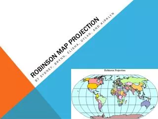
Robinson’s projection “The Robinson projection is neither conformal nor equal-area but a compromise between the two”. Robinson, et al., 1995 Map Scale and Projections

Space oblique Mercator The central line of the space oblique Mercator projection is slightly curved and oblique to the equator. It crosses the polar area at about 81°N and S latitude. Along this line, which represents the Landsat ground-track, the SF is essentially 1.0. The conceptual basis for the projection is similar to that of the transverse Mercator projection, but the central line is not a great circle. From Robinson, et al., 1995 Map Scale and Projections

Map Scale and Projection