PTAS via Local Search
500 likes | 871 Vues
PTAS via Local Search. Rom Aschner and Or Caspi. Outline. Today you will see PTAS for: Geometric Minimum Hitting Set Terrain Guarding Maximum Independent Set of Pseudo Disks Minimum Dominating Set of Disk Graphs

PTAS via Local Search
E N D
Presentation Transcript
PTAS via Local Search Rom Aschner and Or Caspi
Outline • Today you will see PTAS for: • Geometric Minimum Hitting Set • Terrain Guarding • Maximum Independent Set of Pseudo Disks • Minimum Dominating Set of Disk Graphs • Using the technique discovered independently by Har-Peled & Chan (2009) and Mustafa & Ray (2009)
Minimum hitting set problem Mustafa and Ray, 2009
Minimum hitting set problem • Given a range space , • The goal: compute the smallest that has non empty intersection with each • NP-Hard to approximate within a factor of
Minimum hitting set problem • For many geometric range spaces the problem remains NP-hard. • For example: • P – set of points, D – set of unit disks
Minimum hitting set problem • For many geometric range spaces the problem remains NP-hard. • For example: • P – set of points, D – set of disks
Minimum hitting set problem • For many geometric range spaces the problem remains NP-hard. • For example: • P – set of points, H – set of half-spaces in .
Minimum hitting set problem • PTAS (Mustafa & Ray, 2009)
The -level local search algorithm • S • While there is a subset of size that can be replaced with subset of size s.t. is a hitting set. • Then preform the swap • Else, halt. Example:
The -level local search algorithm • Running Time: • The number of iterations is bounded by . • There are at most different local improvements to verify. • Checking whether a certain local improvement is possible takes . • The overall running time is
Approximation Analysis • - the set of points in the optimal solution • - the set of points in the algorithm’s output • Assume: • We want to prove that
We will see that • Thus
Locality condition • satisfies the locality condition if for any two disjoint subsets , it is possible to construct a planar bipartite graph s.t. for any , if and , then there exists two vertices and such that .
Locality condition in disks • The planar bipartite graph is the Delaunay Triangulation of without monochromatic edges.
Locality condition in our graph • For each disk , if and , then there exists two vertices and such that . The locality condition holds !!
Locality condition • Lemma: for any , is a hitting set of • Proof: • If is only hit by the blue points in then one of them has red neighbor that hits • Otherwise, is hit by some point in
Approximation Analysis • - the set of points in the optimal solution • - the set of points in the algorithm’s output • satisfies the locality condition • We want to prove that • The proof is based on the “Separation lemma” (Fredrickson 1987)
Separation lemma • Separation lemma (Fredrickson 1987): For any planar graph and a parameter , we can find a set of size at most and partition of into sets satisfying: • for
Separation lemma • Example : • Then, we can find a set of size at most and a partition of into sets satisfying: • for
Approximation Analysis • How can this separation lemma help us ?? • We have a planar graphof • This graph can be separated into disjoint subsets • Next, we will see that by choosing the correct value of the number of blue points inside each subset is not too big than the number of red points. • Using this observation, we will get that |
Approximation Analysis From the locality condition lemma: If is a hitting set of X then is also a hitting set of X • Let and • Applying we have: • Assume, • replace with – contradiction.
Approximation Analysis • Therefore, • , and large enough constant
-approximation • We proved the following theorem: • Let be a set of points and a set of disks. Then a -level local search algorithm returns a hitting set of size at most in Time. • True also for different regions, such as: • Same height rectangles • Translates of convex shapes • …
Terrain Guarding Gibson, Kanade, Krohn and Varadarajan, 2009
Terrain Guarding • Terrain • A polygonal chain in the plane that is x-monotone.
Terrain Guarding • G: Possible Guard locations • X: Target points that need to be guarded
Terrain Guarding • Objective: find smallest subset of guards such that every point is seenby at least one guard
Terrain Guarding • Previous results: • NP-Hard • 4-approximation • Applications: • Placing guards/cameras along borders • Constructing line-of-sight networks for radio broadcasting • Placing street lights along roads • Placing fire trucks on the Carmel mountain • …
The -level local search algorithm • While there is a subset of size that can be replaced with subset of size s.t. guards . • Then preform the swap • Else, halt.
Terrain Guarding via local search • - the set of guards in the optimal solution • - the set of guards in the algorithm’s output • We can assume that • We want to prove that the locality condition holds. • This means we need to find a planar bipartite graph in which for each , there is an edge between guards and that both see . • As before, using the separation lemma on this graph will show that
Construction 1 • - the leftmost guard that sees among points in • For every guard, we shoot a ray upwards. Let be the first segment in A1 that it hits. v1 x3 v3 x1 v2 x2 v5 v4
Construction 1 • Why are there no crossing edges? • Thanks to the ‘order claim’:Let be four points on the terrain in increasing order according to -coordinate. If sees and sees • Then sees . A D B C
Construction 2 - The flip • Create and in the same way, using the rightmost guards • What if the new edges cross the previous ones? v1 x3 v3 x1 v2 x2 v5 v4
Construction 3 • Finally, for every point x, add an edge in if they are of opposite colors. • Embed this edge along and to remain planar. • The final graph is , planar bipartite. v1 x3 v3 x1 v2 x2 v5 v4
Locality condition • Still need to show that the locality condition holds: For every point there are guards and that both see and they are connected in G. • If and are of opposite colors, we are done because they are connected in . x
Locality condition • Otherwise, assume w.l.g. there are only guards to the left of , and that is red. • Since both and guard , there is also a blue guard that sees , call the leftmost one . • Because is between and , is above . • If it also the first such segment, then x b
Locality condition • Otherwise, let be the first segment in above . • From the order claim on sees. • From the choice of as the leftmost blue guard that sees , is red! x y b
Independent Set Chan & Har-Peled, 2009
Max Independent Set of Pseudo Disks • A set of objects is a collection of pseudo-disks, if the boundary of every pair of them intersects at most twice.
Max Independent Set of Pseudo Disks • Intersection graph – there is an edge between two pseudo-disks if they intersect
Max Independent Set of Pseudo Disks • Max independent set– no pair of objects intersect
Max Independent Set of Pseudo Disks • The bipartite graph is simply the Intersection graph of • Is it planar ? Yes • Embed the edgesalong the intersections • Locality condition ? Yes • If any two red-blue pseudo disks intersect then
Dominating Set Gibson & Pirwani, 2010
Min. Dominating Set of Disk Graphs • Intersection graph – there is an edge between to points if their disks intersect
Min. Dominating Set of Disk Graphs • Minimum Dominating Set - the smallest subset s.t. each vertex is either in or is adjacent to vertex in
More ? Probably yes….