JPEG Image Compression Overview: Efficient Lossy Encoding
Explore the JPEG image compression standard developed by the Joint Photographic Experts Group (JPEG), focusing on the Discrete Cosine Transform (DCT), quantization, and entropy coding. Understand the key observations for effective compression and the main steps involved in the JPEG compression process. Learn about luminance and chrominance quantization tables, the role of DCT on image blocks, and the use of run-length encoding and Differential Pulse Code Modulation (DPCM) in JPEG. Enhance your understanding of efficient lossy encoding methods for digital images with the JPEG standard.

JPEG Image Compression Overview: Efficient Lossy Encoding
E N D
Presentation Transcript
Chapter 9Image Compression Standards 9.1 The JPEG Standard 9.2 The JPEG2000 Standard 9.3 The JPEG-LS Standard 9.4 Bi-level Image Compression Standards 9.5 Further Exploration Li & Drew
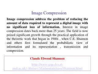
9.1 The JPEG Standard • • JPEG is an image compression standard that was developed by the “Joint Photographic Experts Group”. JPEG was formally accepted as an international standard in 1992. • • JPEG is a lossy image compression method. It employs a transform coding method using the DCT (Discrete Cosine Transform). • • An image is a function of i and j (or conventionally x and y) in the spatial domain. The 2D DCT is used as one step in JPEG in order to yield a frequency response which is a function F(u, v) in the spatial frequency domain, indexed by two integers u and v. Li & Drew
Observations for JPEG Image Compression • • The effectiveness of the DCT transform coding method in JPEG relies on 3 major observations: • Observation 1: Useful image contents change relatively slowly across the image, i.e., it is unusual for intensity values to vary widely several times in a small area, for example, within an 8×8 image block. • • much of the information in an image is repeated, hence “spatial redundancy”. Li & Drew
Observations for JPEG Image Compression(cont’d) • Observation 2: Psychophysical experiments suggest that humans are much less likely to notice the loss of very high spatial frequency components than the loss of lower frequency components. • • the spatial redundancy can be reduced by largely reducing • the high spatial frequency contents. • Observation 3: Visual acuity (accuracy in distinguishing closely spaced lines) is much greater for gray (“black and white”) than for color. • • chromasubsampling (4:2:0) is used in JPEG. Li & Drew
9.1.1 Main Steps in JPEG Image Compression • • Transform RGB to YIQ or YUV and subsample color. • • DCT on image blocks. • • Quantization. • • Zig-zag ordering and run-length encoding. • • Entropy coding. Li & Drew
DCT on image blocks • • Each image is divided into 8 × 8 blocks. The 2D DCT is applied to each block image f(i, j), with output being the DCT coefficients F(u, v) for each block. • • Using blocks, however, has the effect of isolating each block from its neighboring context. This is why JPEG images look choppy (“blocky”) when a high compression ratio is specified by the user. Li & Drew
Quantization • (9.1) • • F(u, v) represents a DCT coefficient, Q(u, v) is a “quantization matrix” entry, and represents the quantizedDCT coefficients which JPEG will use in the succeeding entropy coding. • – The quantization step is the main source for loss in JPEG compression. • – The entries of Q(u, v) tend to have larger values towards the lower right corner. This aims to introduce more loss at the higher spatial frequencies — a practice supported by Observations 1 and 2. • – Table 9.1 and 9.2 show the default Q(u, v) values obtained from psychophysical studies with the goal of maximizing the compression ratio while minimizing perceptual losses in JPEG images. Li & Drew
16 11 10 16 24 40 51 61 12 12 14 19 26 58 60 55 14 13 16 24 40 57 69 56 14 17 22 29 51 87 80 62 18 22 37 56 68 109 103 77 24 35 55 64 81 104 113 92 49 64 78 87 103 121 120 101 72 92 95 98 112 100 103 99 • Table 9.1 The Luminance Quantization Table • Table 9.2 The Chrominance Quantization Table 17 18 24 47 99 99 99 99 18 21 26 66 99 99 99 99 24 26 56 99 99 99 99 99 47 66 99 99 99 99 99 99 99 99 99 99 99 99 99 99 99 99 99 99 99 99 99 99 99 99 99 99 99 99 99 99 99 99 99 99 99 99 99 99 Li & Drew
An 8 × 8 block from the Y image of ‘Lena’ • Fig. 9.2: JPEG compression for a smooth image block. 515 65 -12 4 1 2 -8 5 -16 3 2 0 0 -11 -2 3 -12 6 11 -1 3 0 1 -2 -8 3 -4 2 -2 -3 -5 -2 0 -2 7 -5 4 0 -1 -4 0 -3 -1 0 4 1 -1 0 3 -2 -3 3 3 -1 -1 3 -2 5 -2 4 -2 2 -3 0 F(u, v) Li & Drew
Fig. 9.2 (cont’d): JPEG compression for a smooth image block. Li & Drew
Another 8 × 8 block from the Y image of ‘Lena’ • Fig. 9.2: JPEG compression for a smooth image block. -80 -40 89 -73 44 32 53 -3 -135 -59 -26 6 14 -3 -13 -28 47 -76 66 -3 -108 -78 33 59 -2 10 -18 0 33 11 -21 1 -1 -9 -22 8 32 65 -36 -1 5 -20 28 -46 3 24 -30 24 6 -20 37 -28 12 -35 33 17 -5 -23 33 -30 17 -5 -4 20 F(u, v) Li & Drew
Fig. 9.3 (cont’d): JPEG compression for a textured image block. Li & Drew
Run-length Coding (RLC) on AC coefficients • • RLC aims to turn the values into sets {#-zeros-to-skip, next non-zero value}. • • To make it most likely to hit a long run of zeros: a zig-zag scan is used to turn the 8×8 matrix into a 64-vector. • Fig. 9.4: Zig-Zag Scan in JPEG. Li & Drew
DPCM on DC coefficients • • The DC coefficients are coded separately from the AC ones. Differential Pulse Code modulation (DPCM)is the coding method. • • If the DC coefficients for the first 5 image blocks are 150, 155, 149, 152, 144, then the DPCM would produce 150, 5, -6, 3, -8, assuming di = DCi+1 − DCi, and d0 = DC0. Li & Drew
Entropy Coding • • The DC and AC coefficients finally undergo an entropy coding step to gain a possible further compression. • • Use DC as an example: each DPCM coded DC coefficient is represented by (SIZE, AMPLITUDE), where SIZE indicates how many bits are needed for representing the coefficient, and AMPLITUDE contains the actual bits. • • In the example we’re using, codes 150, 5, −6, 3, −8 will be turned into • (8, 10010110), (3, 101), (3, 001), (2, 11), (4, 0111) . • • SIZE is Huffman coded since smaller SIZEs occur much more often. AMPLITUDE is not Huffman coded, its value can change widely so Huffman coding has no appreciable benefit. Li & Drew
Table 9.3 Baseline entropy coding details – size category. Li & Drew
9.1.2 Four Commonly Used JPEG Modes • • Sequential Mode — the default JPEG mode, implicitly assumed in the discussions so far. Each graylevel image or color image component is encoded in a single left-to-right, top-to-bottom scan. • • Progressive Mode. • • Hierarchical Mode. • • Lossless Mode — discussed in Chapter 7, to be replaced by JPEG-LS (Section 9.3). Li & Drew
Progressive Mode • Progressive JPEG delivers low quality versions of the image quickly, followed by higher quality passes. • Spectral selection: Takes advantage of the “spectral” (spatial frequency spectrum) characteristics of the DCT coefficients: higher AC components provide detail information. • Scan 1: Encode DC and first few AC components, e.g., AC1, AC2. • Scan 2: Encode a few more AC components, e.g., AC3, AC4, AC5. • ... • Scan k: Encode the last few ACs, e.g., AC61, AC62, AC63. Li & Drew
Progressive Mode (Cont’d) • 2. Successive approximation: Instead of gradually encoding spectral bands, all DCT coefficients are encoded simultaneously but with their most significant bits (MSBs) first. • Scan 1: Encode the first few MSBs, e.g., Bits 7, 6, 5, 4. • Scan 2: Encode a few more less significant bits, e.g., Bit 3. • ... • Scan m: Encode the least significant bit (LSB), Bit 0. Li & Drew
Hierarchical Mode • • The encoded image at the lowest resolution is basically a compressed low-pass filtered image, whereas the images at successively higher resolutions provide additional details (differences from the lower resolution images). • • Similar to Progressive JPEG, the Hierarchical JPEG images can be transmitted in multiple passes progressively improving quality. Li & Drew
Encoder for a Three-level Hierarchical JPEG • 1. Reduction of image resolution: • Reduce resolution of the input image f (e.g., 512×512) by a factor of 2 in each dimension to obtain f2 (e.g., 256 × 256). Repeat this to obtain f4 (e.g., 128 × 128). • 2. Compress low-resolution image f4: • Encode f4 using any other JPEG method (e.g., Sequential, Progressive) to obtain F4. • 3. Compress difference image d2: • (a) Decode F4 to obtain . Use any interpolation method to expand to be of the same resolution as f2 and call it E( ). • (b) Encode difference using any other JPEG method (e.g., Sequential, Progressive) to generate D2. • 4. Compress difference image d1: • (a) Decode D2 to obtain ; add it to E( ) to get which is a version of f2 after compression and decompression. • (b) Encode difference using any other JPEG method (e.g., Sequential, Progressive) to generate D1. Li & Drew
Decoder for a Three-level Hierarchical JPEG • 1. Decompress the encoded low-resolution image F4: • – Decode F4 using the same JPEG method as in the encoder to obtain . • 2. Restore image at the intermediate resolution: • – Use to obtain . • 3. Restore image at the original resolution: • – Use to obtain . Li & Drew
9.1.3 A Glance at the JPEG Bitstream Fig. 9.6: JPEG bitstream. Li & Drew
9.2 The JPEG2000 Standard • • Design Goals: • – To provide a better rate-distortion tradeoff and improved subjective image quality. • – To provide additional functionalities lacking in the current JPEG standard. • • The JPEG2000 standard addresses the following problems: • – Lossless and Lossy Compression: There is currently no standard that can provide superior lossless compression and lossy compression in a single bitstream. Li & Drew
– Low Bit-rate Compression: The current JPEG standard offers excellent rate-distortion performance in mid and high bit-rates. However, at bit-rates below 0.25 bpp, subjective distortion becomes unacceptable. This is important if we hope to receive images on our web- enabled ubiquitous devices, such as web-aware wristwatches and so on. • – Large Images: The new standard will allow image resolutions greater than 64K by 64K without tiling. It can handle image size up to 232 − 1. • – Single Decompression Architecture: The current JPEG standard has 44 modes, many of which are application specific and not used by the majority of JPEG decoders. Li & Drew
– Transmission in Noisy Environments: The new standard will provide improved error resilience for transmission in noisy environments such as wireless networks and the Internet. • – Progressive Transmission: The new standard provides seamless quality and resolution scalability from low to high bit-rate. The target bit-rate and reconstruction resolution need not be known at the time of compression. • – Region of Interest Coding: The new standard allows the specification of Regions of Interest (ROI) which can be coded with superior quality than the rest of the image. One might like to code the face of a speaker with more quality than the surrounding furniture. Li & Drew
– Computer Generated Imagery: The current JPEG standard is optimized for natural imagery and does not perform well on computer generated imagery. • – Compound Documents: The new standard offers metadata mechanisms for incorporating additional non-image data as part of the file. This might be useful for including text along with imagery, as one important example. • • In addition, JPEG2000 is able to handle up to 256 channels of information whereas the current JPEG standard is only able to handle three color channels. Li & Drew
Properties of JPEG2000 Image Compression • • Uses Embedded Block Coding with Optimized Truncation (EBCOT) algorithm which partitions each subband LL, LH, HL, HH produced by the wavelet transform into small blocks called “code blocks”. • • A separate scalable bitstream is generated for each code block ⇒ improved error resilience. • Fig. 9.7: Code block structure of EBCOT. Li & Drew
Main Steps of JPEG2000 Image Compression • • Embedded Block coding and bitstream generation. • • Post compression rate distortion (PCRD) optimization. • • Layer formation and representation. Li & Drew
Embedded Block Coding and Bitstream Generation • Bitplane coding. • 2. Fractional bitplane coding. Li & Drew
1. Bitplane Coding • • Uniform dead zone quantizers are used with successively smaller interval sizes. Equivalent to coding each block one bitplane at a time. • Fig. 9.8: Dead zone quantizer. The length of the dead zone is 2δ. Values inside the dead zone are quantized to 0. Li & Drew
• Blocks are further divided into a sequence of 16 × 16 sub-blocks. • • The significance of sub-blocks are encoded in a significance map σP where σp(Bi[j]) denote the significance of sub-block Bi[j]at bitplaneP. • • A quad-tree structure is used to identify the significance of sub-blocks one level at a time. • • The tree structure is constructed by identifying the sub-blocks with leaf nodes, i.e., . The higher levels are built using recursion: , 0 ≤ t ≤ T. Li & Drew
Bitplane Coding Primitives • Four different primitive coding methods that employ context based arithmetic coding are used: • • Zero Coding: Used to code coefficients on each bitplane that are not yet significant. • – Horizontal: • – Vertical: • – Diagonal: Li & Drew
Table 9.4 Context assignment for the zero coding • primitive. Li & Drew
• Run-length coding: Code runs of 1-bit significance values. Four conditions must be met: • – Four consecutive samples must be insignificant. • – The samples must have insignificant neighbors. • – The samples must be within the same sub-block. • – The horizontal index k1 of the first sample must be even. Li & Drew
• Sign coding: Invoked at most once when a coefficients goes from being insignificant to significant. • – The sign bits χi[k] from adjacent samples contains substantial dependencies. • – The conditional distribution of χi[k]is assumed to be the same as −χi[k]. • – is 0 if both horizontal neighbors are insignificant, 1 if at least one horizontal neighbor is positive, or −1 if at least one horizontal neighbor is negative. • – is defined similarly for vertical neighbors. • – If is the sign prediction, the binary symbol coded using the relevant context is . Li & Drew
Table 9.5 Context assignment for the sign coding primitive Li & Drew
• Magnitude refinement: Code the value of given that νi[k] ≥ 2p+1. • – changes from 0 to 1 after the magnitude refinement primitive is first applied to si[k]. • – is coded with context 0 if , with context 1 if and , and with context 2 if . Li & Drew
2. Fractional Bitplane Coding • • Divides code block samples into smaller subsets having different statistics. • • Codes one subset at a time starting with the subset expecting to have the largest reduction in distortion. • • Ensures each code block has a finely embedded bitstream. • • Four different passes are used: forward significance propagation pass ; reverse significance propagation pass ; magnitude refinement pass ; and normalization pass . Li & Drew
Forward Significance Propagation Pass • • Sub-block samples are visited in scan-line order and insignificant samples and samples that do not satisfy the neighborhood requirement are skipped. • • For the LH, HL, and LL subbands, the neighborhood requirement is that at least one of the horizontal neighbors has to be significant. • • For the HH subband, the neighborhood requirement is that at least one of the four diagonal neighbors is significant. Li & Drew
Reverse Significance Propagation Pass • • This pass is identical to except that it proceeds in the reverse order. The neighborhood requirement is relaxed to include samples that have at least one significant neighbor in any direction. • Magnitude Refinement Pass • • This pass encodes samples that are already significant but have not been coded in the previous two passes. Such samples are processed with the magnitude refinement primitive. • Magnitude Refinement Pass • • The value of all samples not considered in the previous three coding passes are coded using the sign coding and run-length coding primitives as appropriate. If a sample is found to be significant, its sign is immediately coded using the sign coding primitive. Li & Drew
Fig. 9.9: Appearance of coding passes and quad tree codes in each block’s embedded bitstream. Li & Drew
Post Compression Rate Distortion(PCRD) Optimization • • Goal: • – Produce a truncation of the independent bitstream of each code block in an optimal way such that distortion is minimized, subject to the bit-rate constraint. • • For each truncated embedded bitstream of code block Bihaving rate with distortion and truncation point ni, the overall distortion of the reconstructed image is (assuming distortion is additive) • (9.3) Li & Drew
• The optimal selection of truncation points ni can be formulated into a minimization problem subject to the following constraint: • (9.5) • • For some λ, any set of truncation point that minimizes • (9.6) • is optimal in the rate-distortion sense. Li & Drew
• The distortion-rate slopes given by the ratios • (9.5) • is strictly decreasing. • • This allows the optimization problem be solved by a simple selection through an enumeration j1 < j2< ... of the set of feasible truncation points. • (9.6) Li & Drew
Layer Formation and Representation • • JPEG2000 offers both resolution and quality scalability through the use of a layered bitstream organization and a two-tiered coding strategy. • • The first tier produces the embedded block bit-streams while the second tier compresses block summary information. • • The quality layer Q1 contains the initial bytes of each code block Bi and the other layers Qq contain the incremental contribution from code block Bi. Li & Drew
Fig. 9.10: Three quality layers with eight blocks each. Li & Drew
Region of Interest Coding in JPEG2000 • • Goal: • – Particular regions of the image may contain important information, thus should be coded with better quality than others. • • Usually implemented using the MAXSHIFT method which scales up the coefficients within the ROI so that they are placed into higher bit-planes. • • During the embedded coding process, the resulting bits are placed in front of the non-ROI part of the image. Therefore, given a reduced bit-rate, the ROI will be decoded and refined before the rest of the image. Li & Drew