Image Compression
Image Compression. Chapter 8. 1 Introduction and background. The problem: Reducing the amount of data required to represent a digital image. Compression is achieved by removing the data redundancies: Coding redundancy Interpixel redundancy Psychovisual redundancy.


Image Compression
E N D
Presentation Transcript
Image Compression Chapter 8
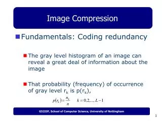
1 Introduction and background • The problem: Reducing the amount of data required to represent a digital image. • Compression is achieved by removing the data redundancies: • Coding redundancy • Interpixel redundancy • Psychovisual redundancy
1 Introduction and background (cont.) • Structral blocks of image compression system. • Encoder • Decoder • The compression ratio where n1 and n2denote the number of information carrying units (usually bits) in the original and encoded images respectively.
1 Introduction and background (cont.) function cr = imratio(f1,f2) %IMRATIO Computes the ratio of the bytes in two images / variables. %CR = IMRATIO( F1 , F2 ) returns the ratio of the number of bytes in %variables / files F1 and F2. IfF1 and F2 are an original and compressed %image, respectively, CR is the compression ratio. error(nargchk(2,2,nargin)); %check input arguments cr = bytes(f1) / bytes(f2); %compute the ratio The Function that finds the compression ratio between two images:
1 Introduction and background (cont.) (cont.) % return the number of bytes in input f. If f is a string, assume that it % is an image filename; if not, it is an image variable. function b = bytes(f) if ischar(f) info = dir(f); b = info.bytes; elseif isstruct(f) b = 0; fields = fieldnames(f); for k = 1:length(fields) b = b + bytes(f.(fields{k})); end else info = whos('f'); b = info.bytes; end
1 Introduction and background (cont.) >> r =imratio( (imread('bubbles25.jpg')), bubbles25.jpg') r = 0.9988 >> f = imread('bubbles.tif'); >> imwrite(f,'bubbles.jpg','jpg') >> r = imratio( (imread( 'bubbles.tif' ) ) , 'bubbles.jpg') r = 14.8578
1 Introduction and background (cont.) • Let denote the reconstructed image. • Two types of compression • Loseless compression: if • Loseless compression: if
1 Introduction and background (cont.) • In lossy compression the error between is defined by root mean square which is given by
1 Introduction and background (cont.) The M- Function that computes e(rms) and displays both e(x,y) and its histogram %COMPARE Computes and displays the error between two matrices. RMSE =COMPARE (F1 , F2, SCALE) returns the root-mean-square error between inputsF1 and F2, displays a histogram of the difference, and displays a scaleddifference image. When SCALE ,s omitted, a scale factor of 1 is used function rmse = compare(f1 , f2 , scale) error(nargchk(2,3,nargin)); if nargin < 3 scale = 1; end %compute the root mean square error e = double(f1) - double(f2); [m,n] = size(e); rmse = sqrt (sum(e(:) .^ 2 ) / (m*n));
1 Introduction and background (cont.) (cont.) %output error image & histogram if an error if rmse %form error histogram. emax= max(abs(e(:))); [h,x]=hist(e(:),emax); if length(h) >= 1 figure; bar(x,h,'k'); %scale teh error image symmetrically and display emax = emax / scale; e = mat2gray(e,[-emax,emax]); figure; imshow(e); end end
1 Introduction and background (cont.) >> r1 = imread('bubbles.tif'); >> r2 = imread('bubbles.jpg'); >> compare(r1, r2,1) >> In E:\matlab\toolbox\images\images\truesize.m (Resize1) at line 302 In E:\matlab\toolbox\images\images\truesize.m at line 40 In E:\matlab\toolbox\images\images\imshow.m at line 168 In E:\matlab\work\matlab_code\compare.m at line 32 ans = 1.5660
1 Introduction and background (cont.) Error histogram
1 Introduction and background (cont.) Error image
2 Coding redundancy • Let nk denotethe number of times that the kth gray level appears in the image and n denote the total number of pixels in the image. The associated probability for the kth gray level can be expressed as
2 Coding redundancy (cont.) • If the number of bits used to represent each value of rk isl(rk), then the average number of bits required to represent each pixel is • Thus the total number of bits required to code an M×N image is MNLavg
2 Coding redundancy (cont.) • When fixed variable length that is l(rk) =m then
2 Coding redundancy (cont.) • The average number of bits requred by Code 2 is
2 Coding redundancy (cont.) How few bits actually are needed to represent the gray levels of an image? Is there a minimum amount of data that is sufficient to describe completely an image without loss information? Information theory provides the mathematical framework to answer these questions.
2 Coding redundancy (cont.) Formulation of generated information Note that if P(E)=1 that is if the event always occurs then I(E)=0 and no information is attributed to it. No uncertainity associated with the event
2 Coding redundancy (cont.) Given a source of random events from the discrete set of possible events with associated probabilities The average information per source output, called the entropy, is
2 Coding redundancy (cont.) If we assume that the histogram based on gray levels is an estimate of the true probability distribution, the estimate of H can be expressed by
1 Introduction and background (cont.) function h = entropy(x,n) %ENTROPY computes a first-order estimate of the entropy of a matrix. %H = ENTROPY(X,N) returns the first-order estimate of matrix X with N %symbols in bits / symbol. The estimate assumes a statistically independent %source characterized by the relative frequency of occurence of the %elements in X error(nargchk(1,2,nargin)); if nargin < 2 n=256; end
1 Introduction and background (cont.) (cont) x = double(x); xh = hist(x(:),n); xh = xh/sum(xh(:)); % make mask to eliminate 0's since log2(0) = -inf i = find(xh); h = -sum(xh(i) .* log2(xh(i))); %compute entropy
1 Introduction and background (cont.) f = [119 123 168 119;123 119 168 168] ; f = [f; 119 119 107 119 ; 107 107 119 119] ; f = 119 123 168 119 123 119 168 168 119 119 107 119 107 107 119 119 p=hist(f(:),8) p = 3 8 2 0 0 0 0 3
1 Introduction and background (cont.) p =p/sum(p) p = Columns 1 through 7 0.1875 0.5000 0.1250 0 0 0 0 0.1875 H = entropy(f) h = 1.7806
Huffman codes • Huffman codes are widely used and very effective technique for compressing data. • We consider the data to be a sequence of charecters.
Huffman codes (cont.) Consider a binary charecter code wherein each charecter is represented by a unique binary string. Fixed-length code: a = 000, b = 001, c = 010, d = 011, e = 100, f = 101 variable-length code: a = 0, b = 101, c = 100, d = 111, e = 1101, f = 1100
Huffman codes (cont.) 100 100 1 0 1 0 55 a:45 a:45 14 86 0 1 0 0 1 58 28 25 30 14 0 0 1 0 1 0 1 0 1 1 a:45 b:13 d:16 d:16 e:9 f:5 c:12 b:13 14 d:16 c:12 0 1 f:5 e:9 Fixed-length code Variable-length code
Huffman codes (cont.) Prefix code: Codes in which no codeword is also a prefix of some other codeword. Encoding for binary code: Example:Variable-length prefix code. a b c Decoding for binary code: Example:Variable-length prefix code.
Constructing Huffman codes • Huffman’s algorithm assumes that Q is implemented as a binary min-heap. • Running time: • Line 2 : O(n) (uses BUILD-MIN-HEAP) • Line 3-8: O(n lg n) (the for loop is executed exactly n-1 times and each heap operation requires time O(lg n) )
Constructing Huffman codes: Example f:5 e:9 c:12 b:13 d:16 a:45 c:12 b:13 d:16 a:45 14 1 0 0 f:5 e:9 14 d:16 25 a:45 0 1 0 0 1 f:5 e:9 c:12 b:13
Constructing Huffman codes: Example a:45 25 30 0 1 0 1 c:12 b:13 d:16 14 0 1 f:5 e:9
Constructing Huffman codes: Example 55 a:45 1 0 30 25 0 0 1 1 d:16 14 c:12 b:13 0 1 f:5 e:9
Constructing Huffman codes: Example 100 1 0 55 a:45 1 0 30 25 0 1 0 1 d:16 14 c:12 b:13 1 0 f:5 e:9
Huffman Codes function CODE = huffman(p) %check the input arguments for reasonableness error(nargchk(1,1,nargin)); if (ndims(p) ~= 2) | (min(size(p))>1)| ~isreal(p)|~isnumeric(p) error('P must be a real numeric vector'); end global CODE CODE = cell(length(p),1); if length (p) > 1 p=p /sum(p); s=reduce(p); makecode(s,[]); else CODE ={'1'}; end;
Huffman Codes(cont.) %Create a Huffman source reduction tree in a MATLAB cell structure byperforming %source symbol reductions until there are only two reducedsymbols remaining function s = reduce(p); s= cell(length(p),1) for i=1:length(p) s{i}=i; end while numel(s) > 2 [p,i] = sort(p); p(2) = p(1) + p(2); p(1) = []; s = s(i); s{2} = {s{1},s{2}}; s(1) = []; end
Huffman Codes(cont.) %Scan the nodes of a Huffman source reduction tree recursively to generate %the indicated variable length code words. function makecode(sc,codeword) global CODE if isa(sc,'cell') makecode(sc{1},[codeword 0]); makecode(sc{2},[codeword 1]); else CODE{sc} = char('0'+codeword); end
Huffman Codes(cont.) >> p = [0.1875 0.5 0.125 0.1875]; >> c = huffman(p) c = '011' '1' '010' '00'
Huffman Encoding >> f2 = uint8 ([2 3 4 2; 3 2 4 4; 2 2 1 2; 1 1 2 2]) f2 = 2 3 4 2 3 2 4 4 2 2 1 2 1 1 2 2 >> whos('f2') Name Size Bytes Class f2 4x4 16 uint8 array Grand total is 16 elements using 16 bytes
Huffman Encoding(cont.) >> c = huffman(hist(double(f2(:)),4)) c = '011' '1' '010' '00' >> h1f2 = c(f2(:))' h1f2 = Columns 1 through 9 '1' '010' '1' '011' '010' '1' '1' '011' '00' Columns 10 through 16 '00' '011' '1' '1' '00' '1' '1'
Huffman Encoding(cont.) >> whos('h1f2') Name Size Bytes Class h1f2 1x16 1018 cell array Grand total is 45 elements using 1018 bytes >> h2f2 = char (h1f2)' h2f2 = 1010011000011011 1 11 1001 0 0 10 1 1 >> whos('h2f2') Name Size Bytes Class h2f2 3x16 96 char array Grand total is 48 elements using 96 bytes
Huffman Encoding(cont.) >> h2f2 = h2f2(:); >> h2f2(h2f2 == ' ') = []; >> whos('h2f2') Name Size Bytes Class h2f2 29x1 58 char array Grand total is 29 elements using 58 bytes
Huffman Encoding(cont.) >> h3f2 = mat2huff(f2) h3f2 = size: [4 4] min: 32769 hist: [3 8 2 3] code: [43867 1944] >> whos('h3f2') Name Size Bytes Class h3f2 1x1 518 struct array Grand total is 13 elements using 518 bytes
Huffman Encoding(cont.) >> hcode = h3f2.code; >> whos('hcode') Name Size Bytes Class hcode 1x2 4 uint16 array Grand total is 2 elements using 4 bytes >> dec2bin(double(hcode)) ans = 1010101101011011 0000011110011000
Huffman Encoding(cont.) >> f = imread('Tracy.tif'); >> c=mat2huff(f); >> cr1 = imratio(f,c) cr1 = 1.2191 >> save SqueezeTracy c; >> cr2 = imratio ('Tracy.tif','SqueezeTracy.mat') cr2 = 1.2627
Huffman Decoding function x = huff2mat(y) % HUFF2MAT decodes a Huffman encoded matrix if ~isstruct(y) | ~isfield(y,'min') | ~isfield(y,'size') | ~isfield(y,'hist') | ~isfield(y,'code') error('The input must be a structure as returned by MAT2HUFF'); end sz = double(y.size); m=sz(1); n= sz(2); xmin = double(y.min) - 32768; map = huffman(double(y.hist)); code = cellstr(char('','0','1')); link = [2; 0; 0]; left = [2 3]; found = 0; tofind = length(map);
Huffman Encoding(cont.) (cont.) while length(left) & (found < tofind) look = find(strcmp(map, code {left(1)})); if look link(left(1)) = -look; left = left (2:end); found = found + 1; else len = length (code); link(left(1)) = len + 1; link = [link; 0; 0]; code{end + 1} = strcat(code{left(1)},'0'); code{end + 1} = strcat(code{left(1)},'1'); left = left(2:end); left = [left len + 1 len + 2]; end end x = unravel (y.code',link, m*n); %Decode using C 'unravel' x = x + xmin - 1; x = reshape(x,m,n);
Huffman Encoding(cont.) (cont.) #include mex.h void unravel (unsigned short *hx, double *link, double *x, double xsz, int hxsz) { int i = 15, j=0, k=0, n=0; while (xsz - k) { if (*(link + n) > 0) { if((*(hx + j) >> i) & 0x0001) n = *(link + n); else n = *(link + n) - 1; if (i) i--; else {j++; i=15;} if( j > hxsz ) mexErrMsgTxt("OutOf code bits??"); }